Iterative SFT (iSFT): dense reward learning

The problem with fine-tuning

When you want a model to do a very specific task, such as following a policy, complying with a tool interface, reasoning in a particular format, obeying safety or business constraints, the easiest thing to do is just fine-tune it on supervised examples of the behaviour you want. This is standard supervised fine-tuning (SFT): collect pairs of (input → ideal output), and train the model to imitate those outputs with next-token prediction.

However, in most realistic settings you don’t actually have ideal outputs to SFT on. You might have a base model that can attempt the task, but it’s pretty bad at it, or it has some ceiling of performance you know you will never exceed. You might have access to a grader (like an LLM-as-a-judge or a verifier), so you can tell whether an answer is good or bad. But you don’t have a clean dataset of perfect demonstrations to imitate. This is a common bottleneck, and plain SFT stalls.

While distillation fine‑tuning can help (SFT’ing on traces generated by a powerful teacher model) this can fall short when even the best models aren’t that good on your specific task. In that case, these distilled outputs aren’t the right targets to imitate. Or even if they are, you are constrained to the performance of the teacher model. Even if you have infinite data, you can only ever converge to the performance of the teacher model.

What people usually try next is RL-style optimisation against that grader. “If I can score an answer, I can reward the model for good answers and punish it for bad ones.” That does work, but it comes with baggage. In particular, the reward is sparse. If the current model output on your task is mostly wrong, you just get “bad,” and there is no learning signal to hillclimb.

So we’re stuck between:

• SFT: needs gold data we don’t have.

• RL: doesn’t need gold data, but is heavier and more brittle than we want for a first pass.

We want something in between:

• As easy/stable as SFT.

• As scalable as RL (no human in the loop for every example).

• And aligned to our task definition, not just “what GPT-5 would have said.”

That’s what iterative SFT gives us.

Iterative SFT

The key observation is that we may not know how to instantly write the perfect answer, we can often recognise when an answer is wrong and often point out how to fix it. For many tasks, we already have:

• an evaluator (”grader”) that can say whether an answer is acceptable, and

• some way to generate revisions conditioned on feedback.

Iterative SFT turns that into training data. The process, step by step:

1. Generate: Start with an input $x$ and have the current model produce an output $y_0$. This first attempts may be garbage.

2. Grade & explain: Run a grader on $y_0$. The grader (LLM-as-judge) doesn’t just say pass/fail; it can also say why it failed (“the chain of thought skipped a step,” “you used the wrong tool call,” “format is invalid,” etc.). So you now have structured feedback.

3. Refine: Use that feedback to produce a new output $y_1$. Re-grade. If it’s still not perfect, repeat: $y_2,y_3,\ldots$

4. Stop when perfect: Once we get an answer $y^*$ that the grader deems fully correct / policy-compliant / format-valid, we save this.

Now we’ve manufactured a clean supervised datapoint $x\rightarrow y^*$.

If we do this across a large batch of inputs, you’ve bootstrapped an SFT-quality dataset without starting from any human-written gold answers. The model’s bad outputs were repaired into good outputs before ever touching the training loop.

We call this process iterative SFT (iSFT).

Relation to DAgger. Conceptually, iSFT mirrors DAgger: the model acts on its own state distribution (prefixes), an expert provides corrections (grader+refiner), and we aggregate those corrections into the SFT corpus, eliminating covariate shift. Unlike classic DAgger, where the expert supplies per-state action labels from a fixed policy, our expert synthesises a sequence-level correction $y^*$ that may rewrite multiple steps. Because refinement can spend extra tokens (more chain-of-thought, tool calls, or structured reasoning) and we can also allow extra tokens at inference, $y^*$ can exceed the performance of any fixed expert policy, effectively scaling quality with compute rather than capping it at the expert’s capabilities. This preserves DAgger’s stability while enabling super-expert targets via “compute-as-supervision”.

Note that in order for this process to work well, we need a very reliable and complete set of evaluators. Otherwise, the accepted datapoints $y^*$ that you end up with may not be good, and you will be fine-tuning on noisy or subpar data (the evaluator may contradict itself, or not be consistent, or be incomplete). Thankfully, we have a process for obtaining such evaluators. We usually rely on strong models like gemini-2.5-pro with maximum thinking to act as LLM-as-a-judge.

By repairing model attempts until they pass the evaluator you actually care about, iSFT can produce training sequences that are higher quality than the sequences generated through pure distillation. This means we can actually outperform any of the closed-source models we care to start with. Here, we’re using our maximally intelligent model to be the grader rather than to generate the answers from scratch, which is a simpler task.

Iterative SFT works

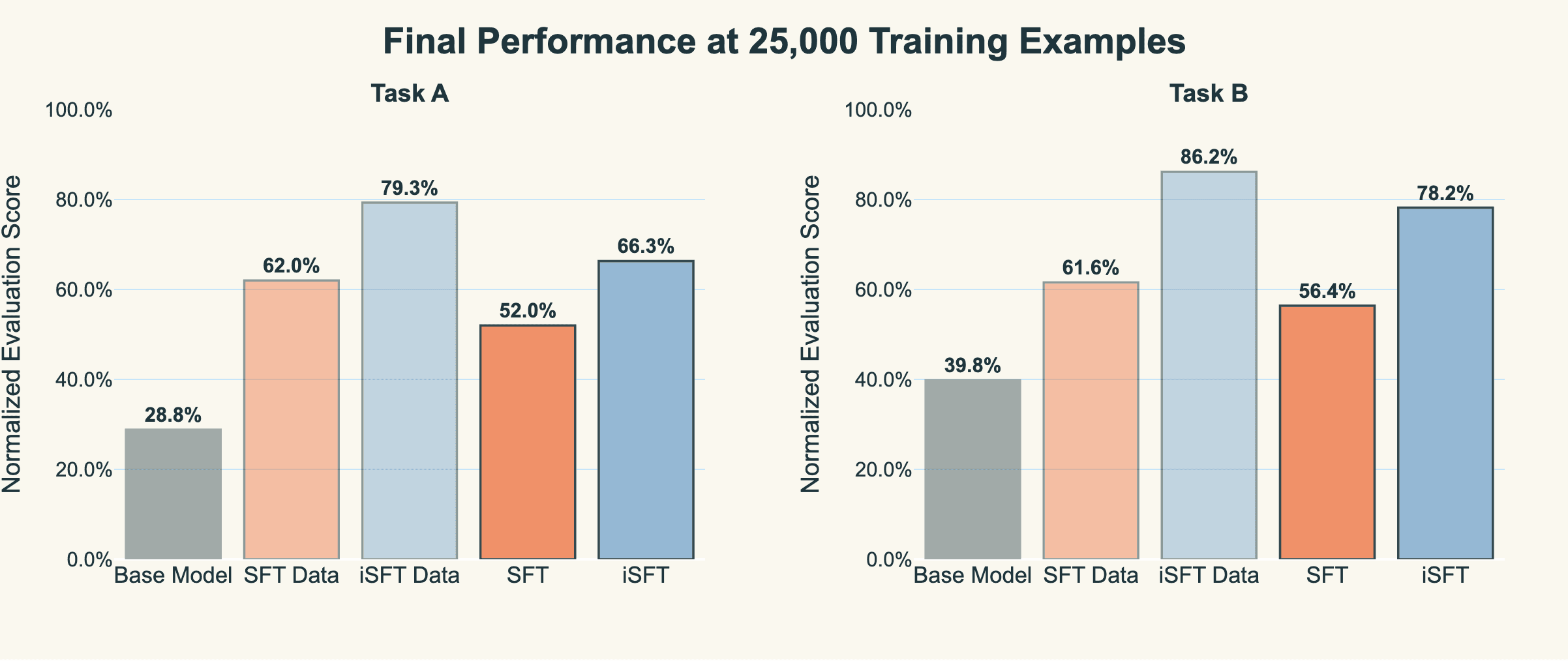
We evaluated iSFT compared to just SFTing on the outputs of gemini-2.5-pro on two real-world medical scribe tasks in active production use: dental clinical notes (Task A) and emergency department notes (Task B). Both tasks use custom graders developed over several weeks with domain experts, scoring outputs on 6-point and 5-point scales respectively. All experiments use gemini-2.5-pro for data generation, evaluation and refinement, and qwen3-32b as the model we're training. We train with LoRA adapters, rank 256, with alpha=32, a constant learning rate (lr=2e-4), and zero LoRA dropout.

At 25,000 training examples, each method plateaus at distinct performance levels: standard SFT achieves 52-56% normalised accuracy, whereas iterative SFT reaches 66-78%, and RGT climbs to 72-83% across both tasks.

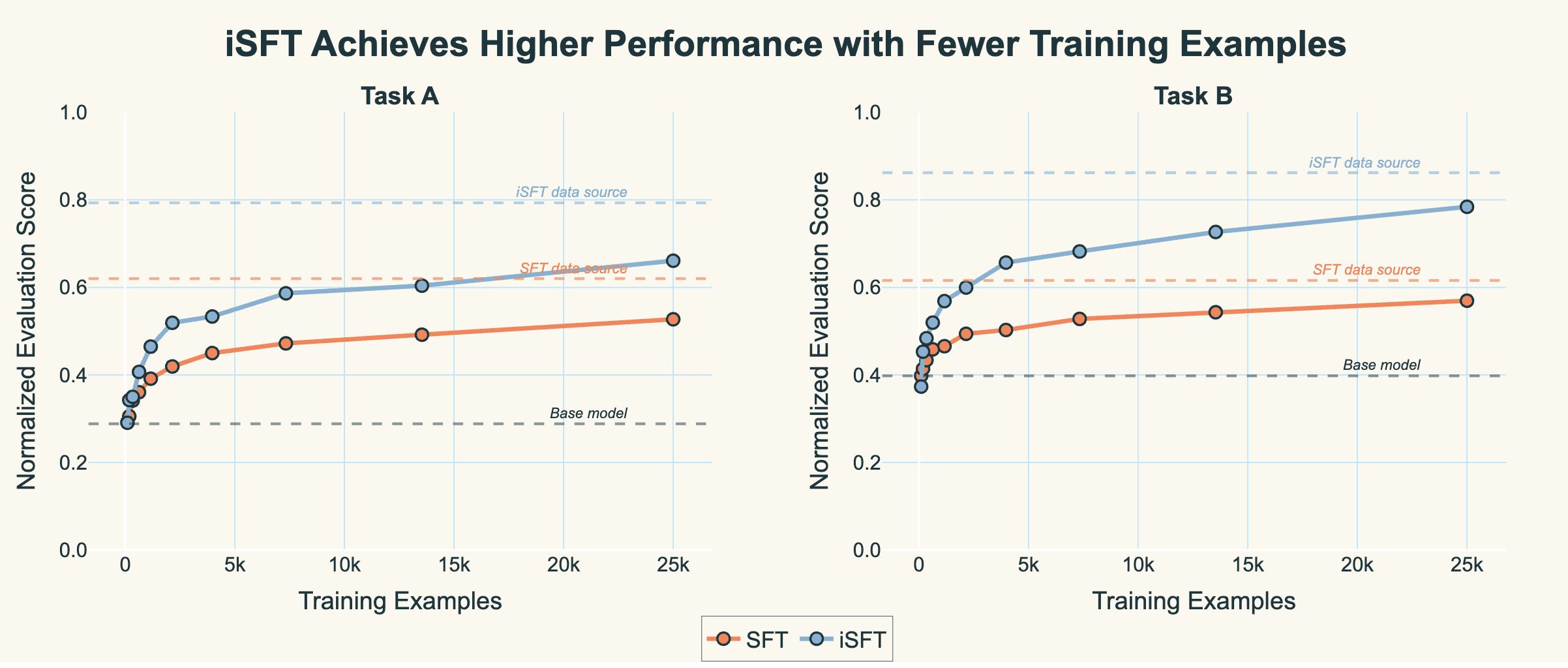
Put more clearly, the scores of the distribution of data we’re training on for iSFT is much higher than the plain SFT data. The actual algorithm that learns the gradient update is the same; the difference is just the quality of data we’re training on.

We can also look at this from a sample efficiency perspective. In terms of actual number of examples we’d need to train on in order to reach a 25% improvement in score, plain SFT requires around 6-7 times more data. We fitted logarithmic growth models to the learning curves and used binary search with linear interpolation to precisely identify where each method crosses this threshold.

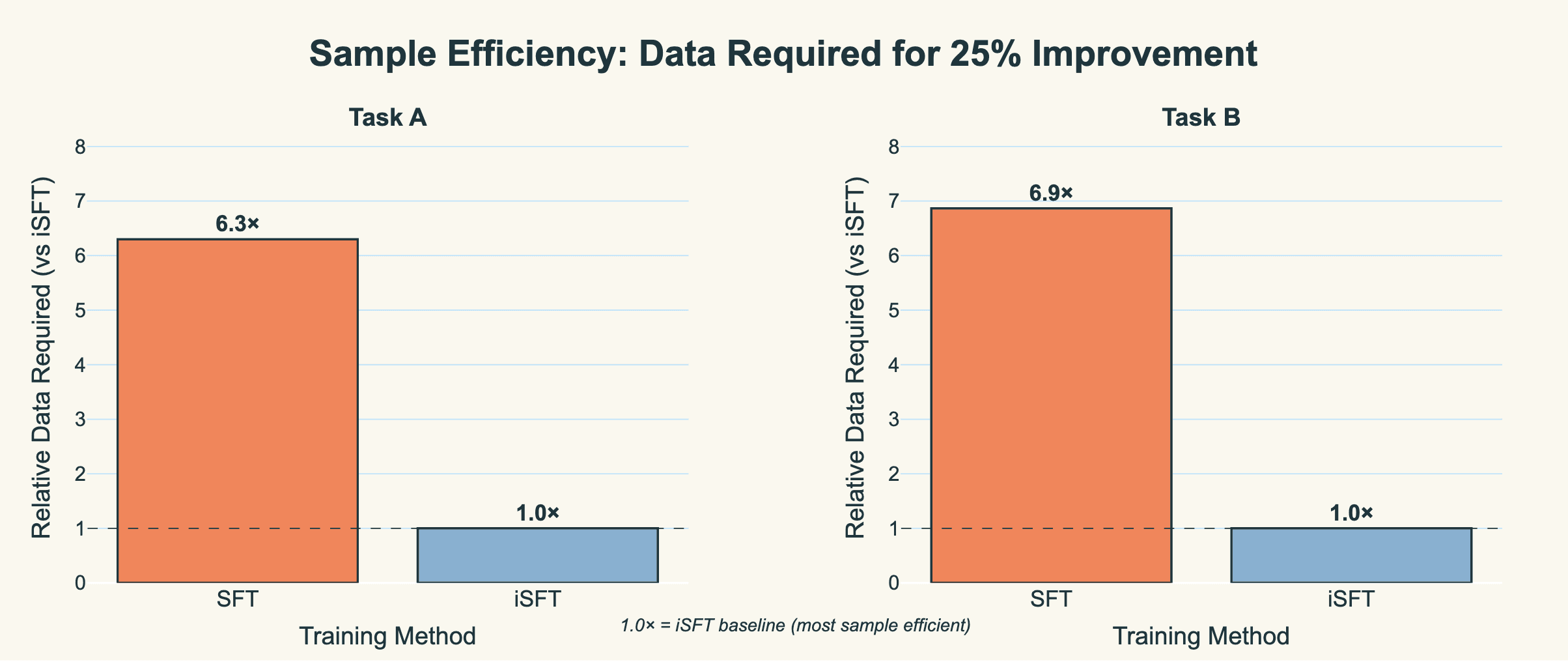
Note this isn’t an entirely fair comparison because we use a lot of tokens in producing the high-quality outputs for iSFT. But it goes to show that if you care about the ceiling of performance, you can get much higher than even the base models with this non-RL approach.

To summarise, iSFT scales monotonically. More data just makes you better.

Because all training pairs are already “perfect” under the grader, you don’t hit the usual plateau where adding more noisy data starts to hurt. You can just generate → refine → absorb into the dataset, over and over. This works with normal supervised training infrastructure: no custom RL loop, no special credit assignment tricks, no weird unstable hyperparameters. You can drop the resulting dataset into any standard SFT pipeline and warm-start a model that’s already close to doing the task, before you do any RL fine-tuning.

iSFT vs RL: the information bandwidth view

We’re going to compare two ways of updating a model from the information-theoretic view, and argue why SFT is much more reward dense and therefore sample efficient. This machine learning folklore is discussed in recent blogposts; see the post by Thinking Machines and the more formal treatment here.

1. Vanilla policy gradient (REINFORCE-style)

   • Sample a rollout from the current model.

   • Score it with a reward signal.

   • Push the policy toward higher-reward behaviour.

2. Iterative SFT

   • Repair the model’s output until it passes our grader oracle.

   • This repaired output is treated as “the correct answer.”

   • Train on it with normal supervised learning.

Both of these are trying to get the model to behave like some desired target policy.

Let’s formalise LLM generation as an MDP. At time-step $t$, the state $s_t$ is the prefix so far, and the action $a_t$ is the next token. The chosen action (the next token) deterministically updates the state (the next token gets appended to the existing prefix). Let’s assume the reward $r_t$ is assigned per token and depends on some unknown parameters like human preferences or objectives. The reward induces an optimal policy \pi^*(a|s). Our current model is a policy $\pi_\theta(a|s)$ which is called at each generation step. An answer of length $T$ is a trajectory $\tau=(s_0,a_0,s_1,a_1,\ldots,s_T)$. Training is about nudging $\pi_\theta$ towards the optimal policy $\pi^*$.

Let’s formalise LLM generation as an MDP. At time-step $t$, the state $s_t$ is the prefix so far, and the action $a_t$ is the next token. The chosen action (the next token) deterministically updates the state (the next token gets appended to the existing prefix). Let’s assume the reward $r_t$ is assigned per token and depends on some unknown parameters like human preferences or objectives. The reward induces an optimal policy $\pi^(a|s)$. Our current model is a policy $\pi_\theta(a|s)$ which is called at each generation step. An answer of length $T$ is a trajectory $\tau=(s_0,a_0,s_1,a_1,\ldots,s_T)$. Training is about nudging $\pi_\theta$ towards the optimal policy $\pi^*$.

So when we talk about “information” here we mean: how many bits of information about $\pi^*$ can the model see from one training example?

In basic policy gradient, the loop is:

1. Sample a full trajectory $\tau\sim\pi_\theta$.

2. Score that entire trajectory with a scalar reward $R(\tau)$

3. Form a gradient update $g=\nabla_\theta \log p_\theta(\tau) \cdot A(\tau)$

where $A(\tau)$ is an advantage term derived from the trajectory return $R(\tau)$, e.g. $A(\tau)=R(\tau)-b$ for some baseline $b$.

Given that the gradient $g$ is what is observed by our model, an important consequence follows. One can make some arguments to conclude that in this expression, all information about the learning task flows through the scalar $A(\tau)$.

In particular, if we condition on the history $\mathcal{H}$ up to this point, then $\tau\perp\pi^*\mid\mathcal{H}$ and $\nabla_\theta\log p_\theta(\tau) = \sum_{t=0}^{T-1}\nabla_\theta \log\pi_\theta(a_t|s_t)$ is fully determined by the current model $\theta$ and gives no information about the target policy. The information the model can get from the gradient $I(g;\pi^*|\mathcal{H})$ is therefore upper-bounded by the entropy of this advantage scalar $H(A|\mathcal{H},\tau)$. In our modelling setup, if we assume this advantage is calculated via a trajectory return $\sum_{t=0}^{T-1}\gamma^t r_t$ that collapses the rewards at each time-step to a single value, this vastly reduces the amount of information the model can get from one rollout.

Indeed, if one assumes some reasonable “finite resolution” of this return scalar (different reward sequences are collapsed into the same total return, the finite resolution of the scalar itself etc) this quite literally caps the amount of information obtainable from one rollout to a few handfuls of bits — $O(1)$ in the sequence length.

This gives a sense of why vanilla policy gradient is sample-hungry. You burn lots of rollouts to get a tiny trickle of information about what good behaviour is, having collapsed a potentially rich set of rewards into a low bandwidth pipe into the model. It also hints at the credit assignment problem: the model just gets told “bad,” not “bad specifically at step $t$ when you made the illegal tool call”.

Now let’s look at iterative SFT in the same frame. Assuming that our refinement evaluators are strong and will only accept perfect completions, we can treat our $y^*$ as a gold standard supervised training example that contains a denser reward higher-dimensional reward signal. Concretely, a reasonable approximation for this kind of supervised learning is to treat each state–action pair along this “approved” trajectory, $(s_t^*,a_t^*)\in y^*$as a labeled datapoint following the optimal policy $\pi^*$.

Then we do standard next-token training, where the gradients become $\nabla_\theta \log p_\theta(y^|x)=\sum_{t=0}^{T-1} \nabla_\theta\log\pi_\theta(a_t^|s_t^*)$. The model now gets dense feedback per step. If the model is still imperfect at this task, then many of those actions $a_t^*$– will differ from what $\pi_\theta$ would have done, which means they’re informative. The “surprise” of the full corrected answer under the current model is $-\sum_{t=0}^{T-1}\log \pi_\theta(a_t^*|s_t^*)$and that scales with sequence length $T$. Given sequences on the order of thousands of tokens or above, one repaired trajectory can convey a much larger $O(T)$ number bits about $\pi^*$, not just a constant handful $O(1)$.

Sample efficiency in practice

Practically, this is why iSFT can get you most of the policy-shaping benefits you want from RL long before you run a single unstable RL step. You front-load dense information about $\pi^*$ instead of trying to extract $\pi^*$ from a trickle of 1-bit thumbs-ups.

In comparing sample efficiency, it's helpful to think about the number of LLM calls required to achieve similar levels of performance.

iSFT approach:

• Generate initial outputs from the model

• Use LLM calls (e.g., Gemini) to evaluate and provide feedback for refinement

• Iteratively refine outputs until they pass evaluation (typically 1-2 refinement rounds)

• Once we have a batch of perfect outputs $y^*$, perform standard supervised fine-tuning

RL with LLM-as-a-judge approach:

• Sample rollouts from the current policy during training

• Use LLM judge to score every single rollout during the RL training loop

• Update policy based on scalar rewards

• Repeat for many thousands of training steps

The key difference: in iSFT, we make LLM calls upfront to create a high-quality dataset, then train efficiently via supervised learning. In RL with LLM-as-a-judge, we must make LLM calls continuously throughout training for every sampled trajectory.

Given our information-theoretic arguments above—that each iSFT example provides $O(T)$ bits of information while each RL rollout provides only $O(1)$ bits—we'd expect RL to require orders of magnitude more LLM judge calls to extract the same amount of information about $\pi^*$. If a typical sequence has $T\approx 1000$ tokens, the ratio can easily be an order of magnitude more LLM calls needed for RL to achieve comparable policy shaping. This makes iSFT not just more stable and easier to implement, but also far more economical in terms of compute and API costs when using powerful models as evaluators.

An alternative approach worth comparing to is "poor man's RL" (also known as rejection sampling). Like iSFT, this method also produces a supervised dataset from model outputs, but uses a different mechanism: instead of refining imperfect outputs, we simply have our model generate many attempts at the task and use a verifier to keep only the ones that pass. This also gives us a set of approved rollouts $y^*$ which we can then use for standard SFT.

While both approaches produce supervised datasets of "good" examples, we expect iSFT to be more sample efficient and to scale much better as the task gets harder relative to the model ability. Rejection sampling can be extremely wasteful when the base model has a low success rate. If your model only succeeds 5% of the time, you need to generate 20 outputs to get one training example. iSFT instead takes failed attempts and repairs them through targeted refinement (typically a handful of rounds). This translates to far fewer LLM calls to build a dataset of the same size. Further, as the task gets harder and the rejection ratio becomes higher, we expect rejection sampling to scale exponentially worse.

Further, rejection sampling is limited to whatever your base model can already produce, as you're essentially filtering for its “lucky” outputs. iSFT actively improves outputs through refinement, which means the final dataset can contain solutions of higher quality than the base model would naturally generate. The refinement process can fix specific errors and inject corrections that pure sampling would struggle to discover.

Of course, neither iSFT nor poor man's RL produces perfect supervised data exactly from the $\pi^*$ policy. Both rely on imperfect evaluators and produce approximations. But iSFT's refinement loop makes better use of each generation attempt and can systematically improve toward $\pi^*$, rather than hoping to stumble upon good examples through repeated sampling.

Future work

We have many directions to explore for improving iSFT further. One key area concerns the choice of evaluator model. Currently, we use a strong model as our evaluator, typically something like gemini-2.5-pro or gpt-5 with maximum thinking budgets, which excels at providing high-quality feedback and refinements. However, there may be advantages to using a more on-policy model instead. If we're training Qwen but using Gemini's responses as our refined targets, we're introducing a potentially large KL divergence between Qwen's base policy and Gemini's generations. This distribution mismatch could make the learning task harder or less stable. In contrast, if we use Qwen itself (or a variant of it) to generate the feedback and refinements, the KL divergence would be much smaller; the refined outputs would be more naturally aligned with what the base model can learn, since they come from a similar policy distribution. This on-policy refinement approach could lead to faster convergence and better final performance.