Research
October 10, 2025
Practical LoRA Research
Fine-tuning at Scale: What LoRA Gets Right (and LoRA-XS Doesn’t).
Authors
Affiliations
Max Kirkby
Parsed
Charles O'Neill
Parsed
At Parsed, we fine-tune language models constantly. It's core to what we do, and we spend considerable time and compute doing it. So anything that reduces training costs without sacrificing quality naturally captures our attention.
Low-rank updates (specifically LoRA and the more recent LoRA-XS, along with all their variants) offer exactly this promise. LoRA's approach is instead of updating all parameters, calculate low-rank updates for each weight matrix and merge them back at the end. LoRA-XS takes this further, initializing low-rank matrices from the truncated SVD of the original matrix, freezing them, and training only a tiny square matrix in between to navigate SVD space.
LoRA cuts trainable parameters by an order of magnitude or more. LoRA-XS reduces them even further. For us, this could mean training much larger models on smaller instances, which is a significant operational advantage if we can match full fine-tuning quality.
Recently, Thinking Machines published research characterizing exactly when LoRA excels. We've been running parallel experiments, but focused on our real-world production tasks: clinical scribing, insurance policy recommendation, and similar domains. Our findings align with Thinking Machines on the core question: LoRA does match full fine-tuning when you get the details right, but we wanted to extend this in two directions.
First, we wanted to confirm that training loss correlates reliably with downstream performance on our robust LLM-as-judge evaluation suites. If this holds, we can use loss to checkpoint runs and only run expensive evaluations at the end. We provide initial analysis here, with deeper investigation planned for future work.
Second, we wanted to test LoRA-XS. The parameter reduction is compelling, potentially another order of magnitude beyond LoRA. Unfortunately, we couldn't replicate the results from the LoRA-XS paper, which claimed it could outperform LoRA at similar rank. After extensive experimentation, we now view LoRA-XS as theoretically well-motivated but practically inferior to both LoRA and full fine-tuning—at least when performance requirements are relatively inelastic. (If you're severely constrained on memory and compute for smaller models, it might still be viable.)
What follows is our analysis of both approaches on production tasks, with particular attention to where LoRA succeeds, where it struggles, and why LoRA-XS fell short of expectations.
Evaluating the performance of LoRA vs full fine-tuning
For this analysis, we fine-tune qwen-3-4B on a clinical scribe task. While matching final loss values should translate to matching evaluation performance, we've empirically found that even small differences in the final negative log-likelihood can lead to significant performance differences on downstream tasks.
First, we validate that training loss converges to approximately the same place for each rank and for full fine-tuning. Figure 1 shows the training curves for 1,000 examples. While full fine-tuning achieves the lowest final loss, the fact that rank1 achieves the second-lowest suggests the differences between curves are likely due to random seeds and initialization noise rather than genuine capacity constraints—at this dataset size, all methods have sufficient capacity.
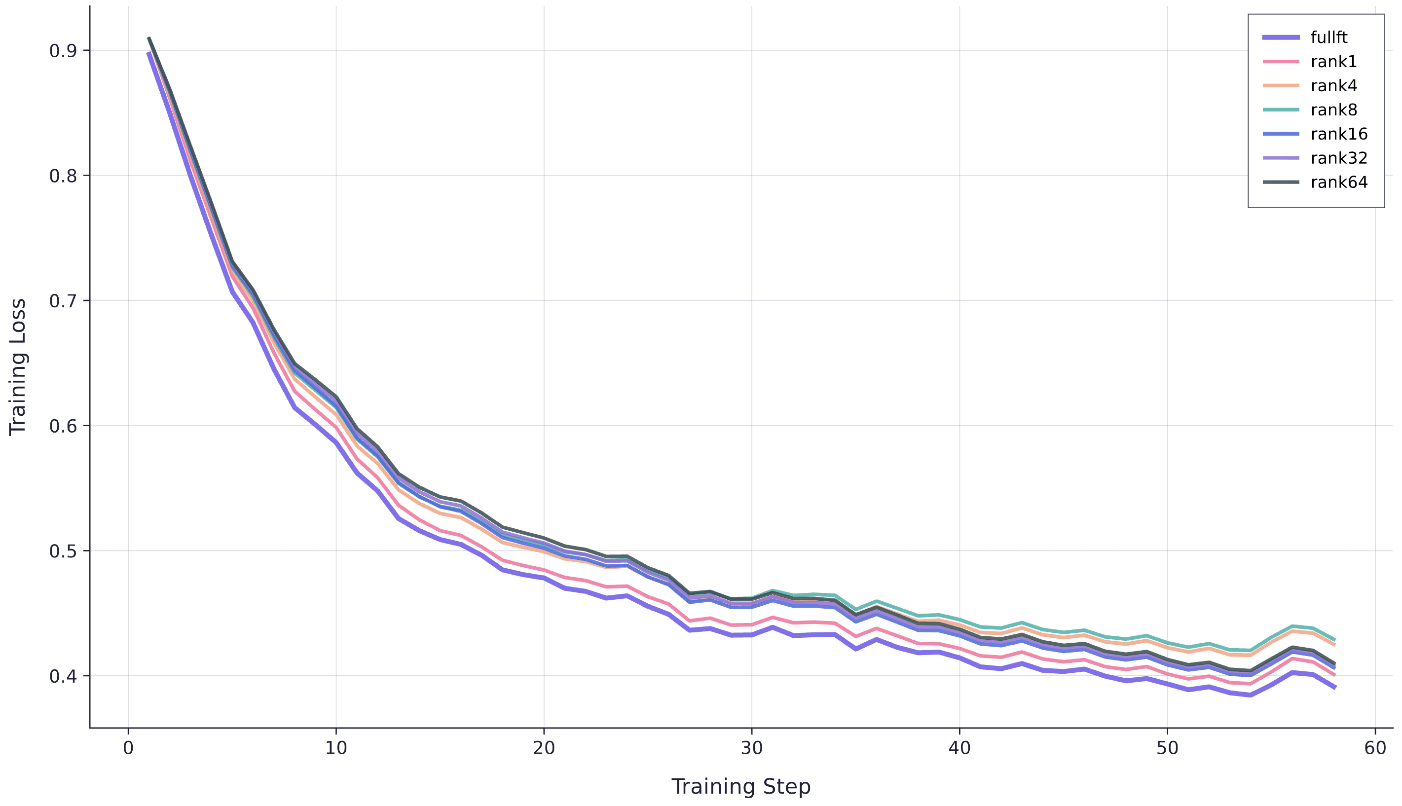
Training loss curves for full fine-tuning and LoRA ranks 1, 4, 8, 16, 32, and 64 on 1,000 clinical scribe examples. All methods converge to similar final loss values, with differences attributable to random variation rather than capacity limitations.
To confirm this, we evaluate each model using our five LLM-as-judge evaluators. Each evaluator examines a model output, generates a rationale, and returns a binary pass/fail judgment (we use gemini-2.5-pro with maximum reasoning tokens). For each example, we sum the five binary scores to get a value from 0-5, then average across all examples to produce a quasi-Likert score.
The figure below shows the results. Pairwise Mann-Whitney U tests (a robust non-parametric test appropriate for Likert-scale data) reveal that most fine-tuning methods perform statistically similarly, with the notable exception of full fine-tuning versus rank4 (p < 0.05). However, this single significant difference appears to be noise rather than a systematic pattern.
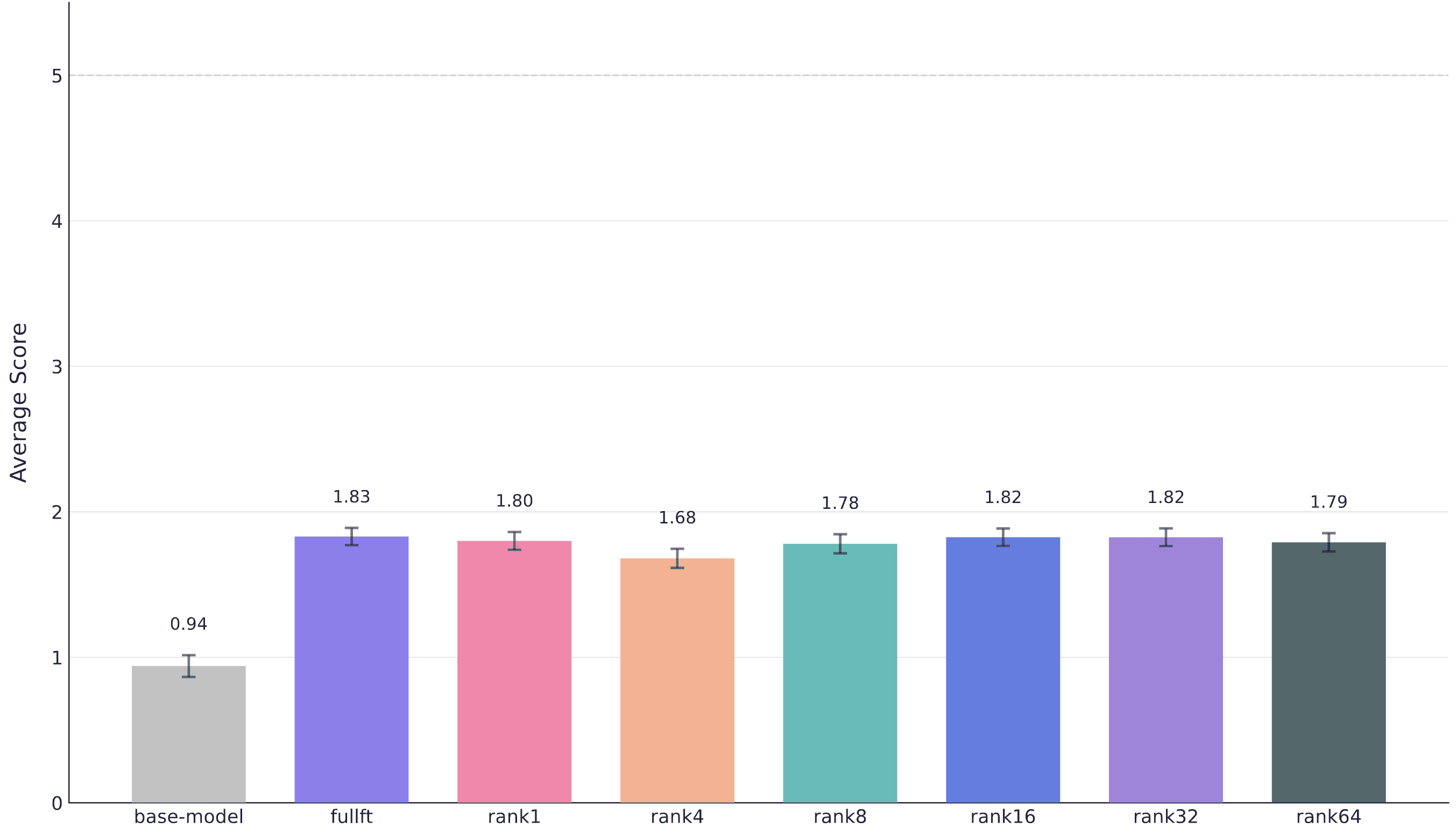
Evaluation scores for different fine-tuning methods on 1,000 examples. Error bars show standard error. Most methods achieve statistically similar performance, clustering around 1.7-1.8 out of 5.
We can also examine the relationship between final training loss and evaluation performance. Figure 3 shows a moderate negative correlation (r = -0.70, R^2 = 0.49), suggesting that lower training loss tends to associate with better downstream performance; approximately 49% of the variance in evaluation scores can be explained by final loss. However, this relationship doesn't reach statistical significance (p = 0.08) at the conventional α = 0.05 threshold, likely due to our limited sample size of seven methods. The trend suggests each 0.1-point reduction in training loss corresponds to an average 0.28-point improvement in evaluation score, but we can't claim this relationship is reliable based on this data alone.
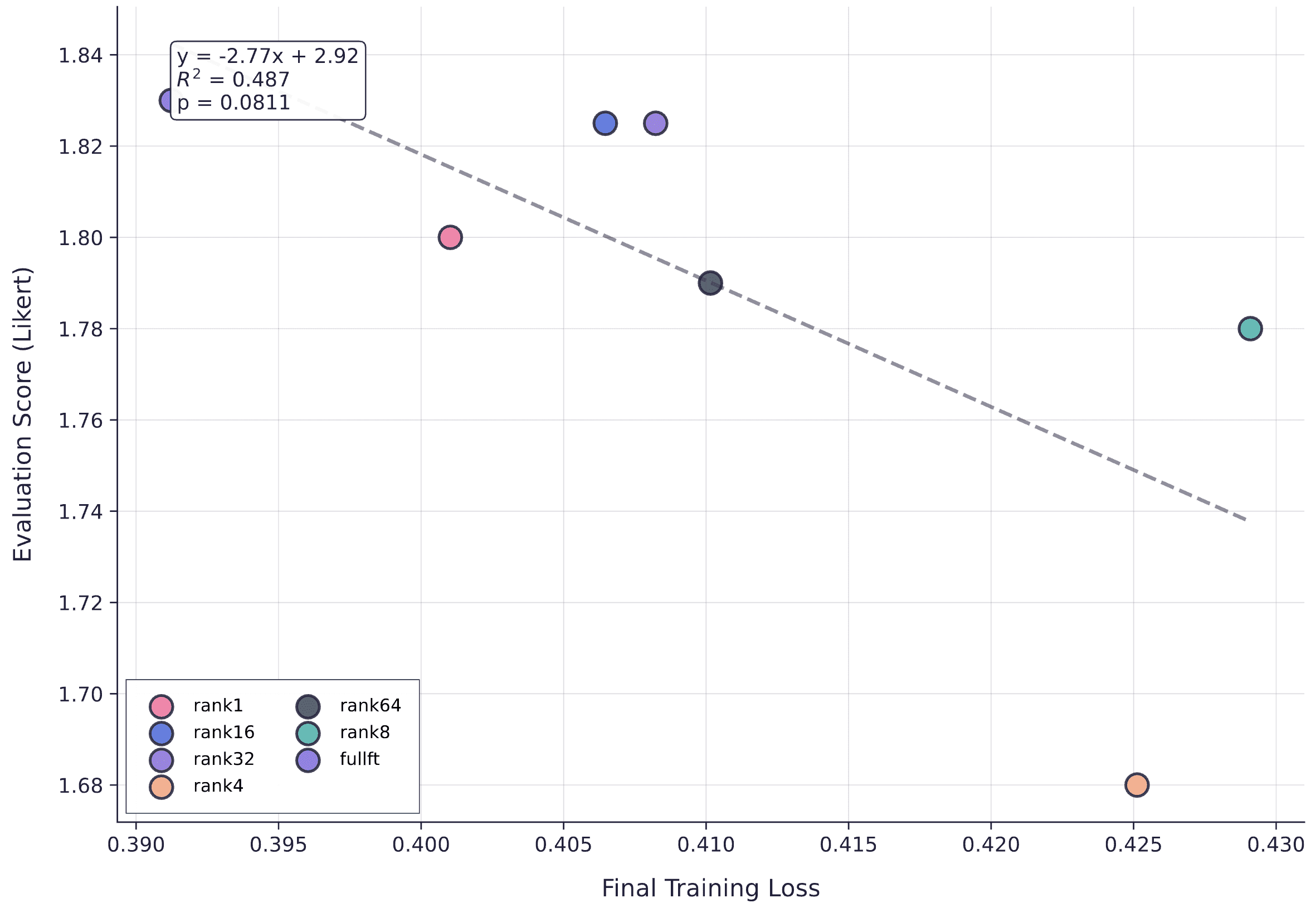
Relationship between average final training loss (last 5 steps) and evaluation performance. The moderate correlation suggests loss could be useful for checkpointing, though the relationship isn't statistically significant with this sample size.
Scaling to larger datasets
The 1,000-example results suggest equivalence across methods, but this could simply reflect that all approaches have sufficient capacity for small datasets. Following Schulman's analysis, we expect low-rank adapters might saturate at larger dataset sizes, where their limited capacity prevents them from keeping pace with higher-rank adapters and full fine-tuning.
To test this, we train models on 1K, 5K, 10K, and 30K examples and evaluate the final checkpoints using the same five-evaluator setup. The figure below shows the results. Evaluation performance scales log-linearly with dataset size, with remarkably consistent improvement curves across methods, which is a satisfying validation of the predictability of fine-tuning at scale.
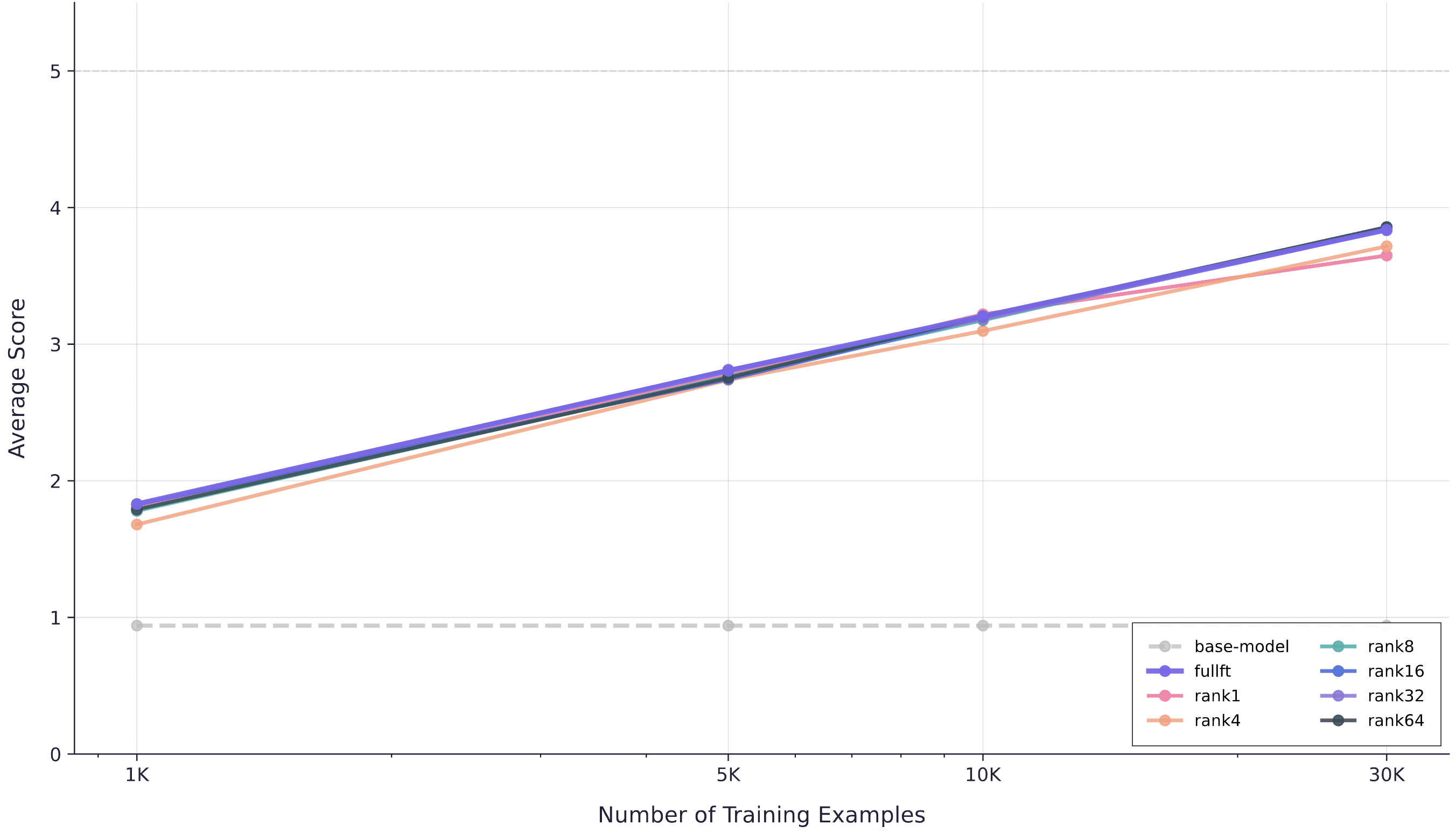
Evaluation performance as a function of training dataset size. Most LoRA ranks track full fine-tuning across all dataset sizes, with rank1 and rank4 showing capacity saturation at 30K examples.
Most LoRA ranks achieve the same performance as full fine-tuning across all dataset sizes, with two exceptions: rank1 and rank4 begin to underperform at 30K examples. This matches Schulman's findings—beyond a certain dataset size, very low-rank adapters no longer have sufficient capacity to match higher-capacity methods. For our clinical scribe task, rank8 and above remain equivalent to full fine-tuning even at 30K examples, while rank4 shows the first signs of capacity saturation. (Note each of these examples contain about 5000 input tokens and 1000 output, so contextualize this as you will.)
This has practical implications: for production systems, using rank8 or rank16 appears to offer the full benefits of LoRA's parameter efficiency without sacrificing quality, at least up to dataset sizes of 30K examples. Only the most aggressive parameter reduction (rank1 and rank4) shows clear degradation.
Capacity analysis
A fundamental question in parameter-efficient fine-tuning is: when do low-rank adapters run out of capacity? Some research suggests language models store approximately 2 bits per parameter (or maybe slightly higher). If each training token contributes roughly 1 bit of information, we might expect LoRA adapters to saturate when the total training tokens reaches twice the number of trainable parameters. More practically: at what rank and dataset size do different LoRA configurations begin to diverge?
To investigate this, we train qwen3-4B and qwen3-8B on a clinical scribe task with 25,000 examples and examine how different ranks behave as training progresses.
Final training loss versus LoRA rank after training on 5,000 examples. Counterintuitively, lower ranks achieve better final loss, suggesting rank1 has begun to saturate while higher ranks are still learning efficiently.
The results are initially counterintuitive. Rank1 achieves the highest final loss, but as rank increases, final loss actually gets worse—the opposite of what capacity theory would predict. What's happening here?
The most likely explanation relates to learning dynamics rather than capacity limits. At 5,000 examples, rank1 has already begun to saturate—it's approaching the point where it can't absorb additional information efficiently. The loss curve for rank1 would start to level off if we continued training. Higher ranks, meanwhile, still have ample capacity and continue learning efficiently at the same learning rate (we use α=32 for all ranks, which affects the effective learning rate). They're still in the steep part of their learning curves, which means they converge faster to lower loss values—but they haven't yet hit their capacity limits.
This suggests a hypothesis: if we train much longer, we should see each rank saturate in sequence, with rank1 saturating first, then rank4, and so on. To test this, we extend training to 25,000 examples (5x more data).
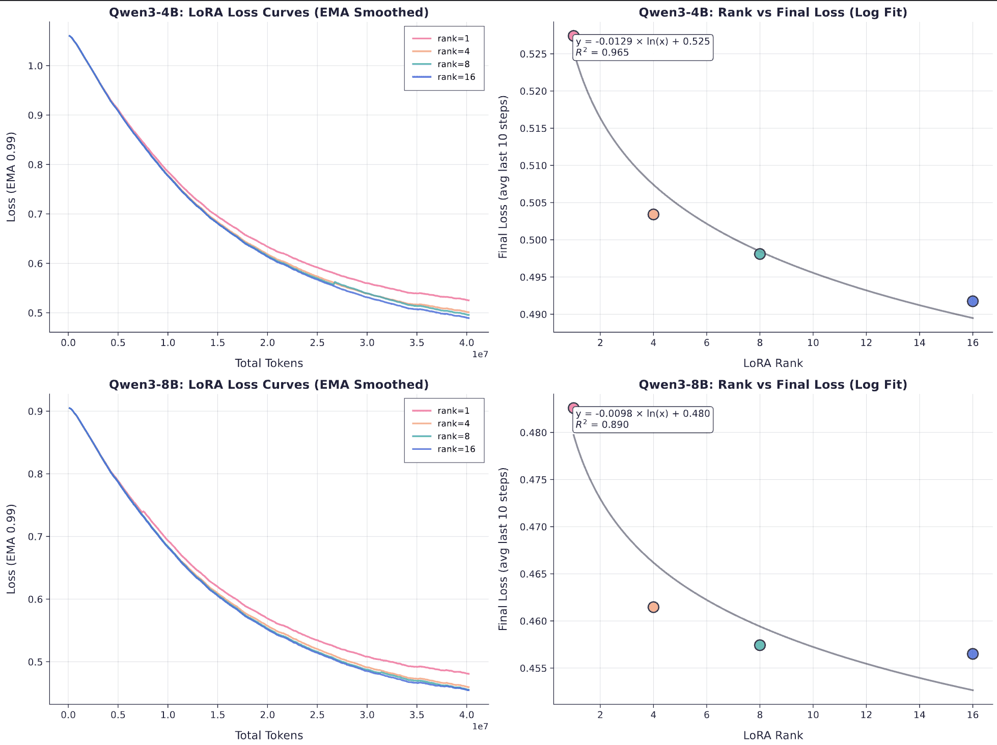
Training curves and final loss versus rank for 25,000 examples on Qwen3-4B (top) and Qwen3-8B (bottom). Left: Loss curves show rank1 trailing other ranks throughout training. Right: Final loss follows a clear logarithmic relationship with rank.
The extended training confirms the hypothesis, but reveals something more structured than simple saturation. Instead, the sample efficiency (ie the rate at which the loss goes down) starts to diverge between different ranks.
The right panels shows that final loss follows a logarithmic relationship with rank. For qwen3-4B, the fit is nearly perfect (R^2 = 0.965): each doubling of rank reduces final loss by approximately 0.009 nats. The 8B model shows the same pattern (R² = 0.890), though with slightly weaker correlation, likely due to the larger model requiring higher ranks to see capacity effects.
This logarithmic relationship means that it’s not simply that low ranks “run out of capacity” at some threshold but rather that capacity scales smoothly with rank according to a predictable function. The consistency across model sizes (4B and 8B) suggests this is an actual property of LoRA's low-rank parameterization rather than an artifact of a particular architecture. It also provides a principled way to select rank: measure the loss-parameter tradeoff on a small training run, then extrapolate to predict how much capacity you'll need for larger datasets. However, this doesn’t necessarily tell you where everything will diverge for large datasets.
For our clinical scribe task at 25K examples, rank4 appears sufficient for the 4B model (final loss ≈ 0.503), while rank8 provides only marginal improvement ($\approx$ 0.498). The logarithmic curve suggests we'd need to push to rank32 or beyond to see another meaningful reduction—an increasingly expensive proposition for diminishing returns.
The evaluation results show saturation, but when exactly does this happen? Looking at training loss across dataset sizes shows that rank1 starts to saturate around 5k, rank4 around 10k. Note that this plot is slightly misleading as we use the actual eval loss at the checkpoint, rather than the smoothed training loss from above. But the point is: higher ranks continue scaling linearly (extrapolated beyond 30k).
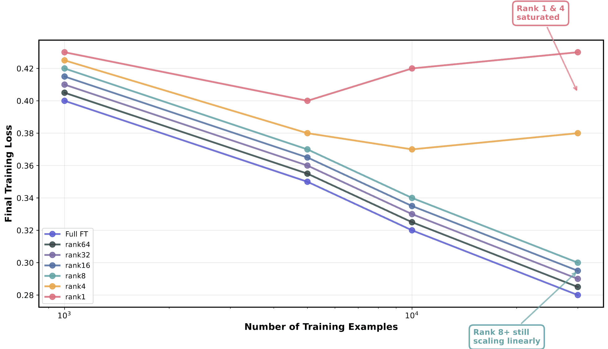
Divergence of LoRA ranks as dataset size increases. Importantly, we start to see some “saturation” (or levelling off) of the lower-rank LoRAs.
Envelope capacity maths
In practice, a simple way to predict when different LoRA ranks will “run out of capacity” is to treat capacity as ~2 bits per trainable parameter and reckon that saturation occurs when total training bits ≈ adapter capacity. With only ~200 tokens per example contributing to loss, the saturation point (in examples) scales linearly with rank because LoRA trainables scale proportional to r:
$\text{examples}_\text{sat}(r)\approx r\cdot\text{examples}_\text{sat}(1)$
Empirically in our scribe runs, very-low ranks (r=1,4) start to lag by ~30k examples, while r≥8 continue to track full FT, consistent with this linear rule and with our observation that final loss decreases roughly logarithmically with rank (each doubling buys a small, predictable drop). Concretely, if you infer from your curves that r=1 saturates around 5k examples, expect r=4≈20k, r=8≈40k, r=16≈80k, etc.; if r=1≈10k, double those numbers. Operationally, pick the smallest rank whose projected saturation point comfortably exceeds your planned dataset size (e.g., r=8–16 up to ~30k examples in our task), remembering that divergence can appear before the hard capacity limit due to optimisation dynamics.
Evaluating the performance of LoRA vs LoRA-XS
For this analysis, we evaluate LoRA against LoRA-XS on a tool-calling task: a customer queries an insurance product, the agent makes tool calls to grep-search a knowledge base of insurance products, receives responses, and generates a compliant answer. We fine-tune qwen3-32B on conversations generated by GPT-5, testing various LoRA and LoRA-XS configurations.
Initial analysis from the LoRA-XS paper
The results from the LoRA-XS paper allow us to estimate roughly (1) how many parameters LoRA-XS needs vs LoRA before it beats it, and (2) what rank LoRA-XS needs vs LoRA in order to beat it. We took the results from this paper and visualized them in three ways to figure out roughly how big (in terms of rank) our LoRA-XS adapters should expect to be if we’re to beat LoRA, considering dataset size and model size (number of trainable params induced by the model).
The efficiency gains are substantial: LoRA-XS reaches 88.69% on GLUE with just 60K parameters versus LoRA's 87.82% with 800K parameters, and achieves 80.5-85.3% on commonsense reasoning with 3.67M parameters versus LoRA's 77.6-80.8% with ~56M parameters.
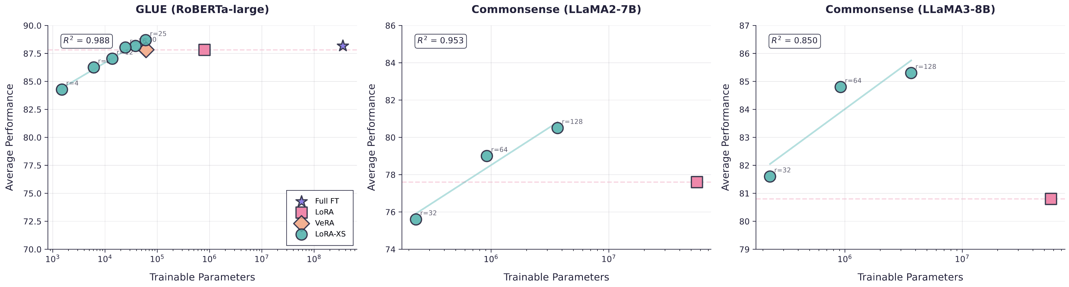
Parameter efficiency frontier across GLUE and commonsense reasoning benchmarks. LoRA-XS achieves superior performance to LoRA while using 10-15× fewer parameters across all tested benchmarks.
LoRA-XS surpasses the LoRA baseline at rank 16-20 for RoBERTa-large, rank 128 for LLaMA2-7B, and at all tested ranks for LLaMA3-8B, with stronger base models requiring lower ranks to match LoRA performance.
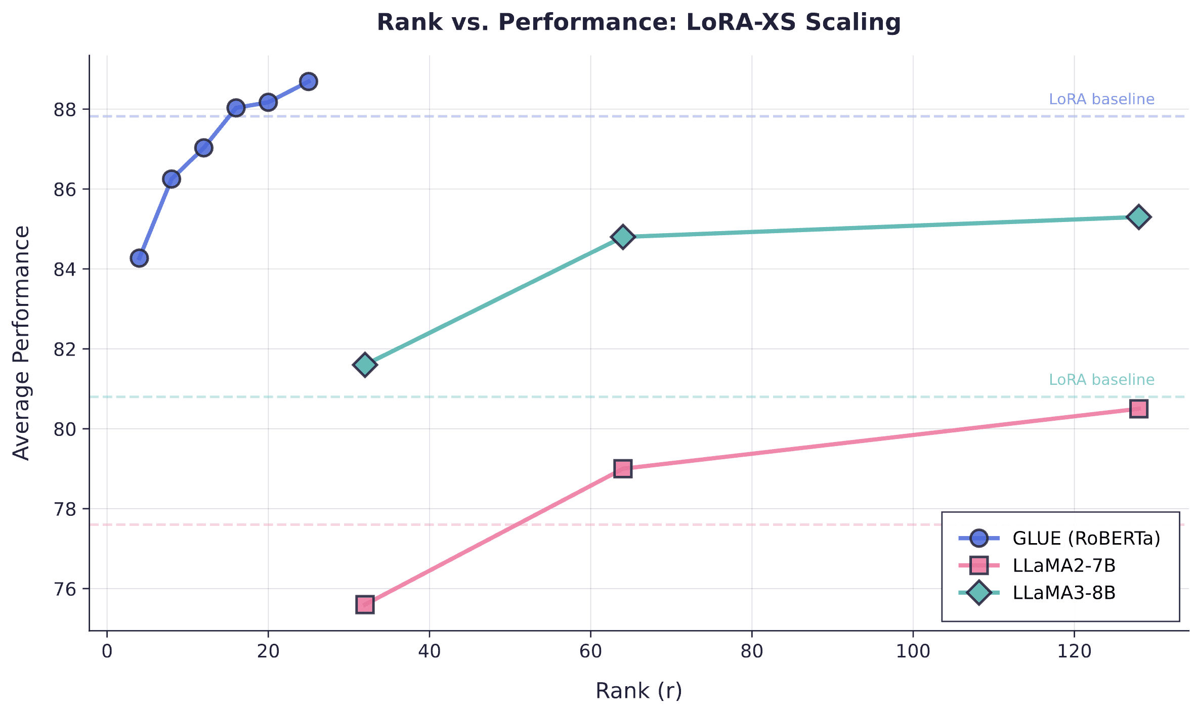
LoRA-XS performance scaling with rank across three benchmarks, with horizontal dashed lines indicating corresponding LoRA baseline performance.
At extremely low budgets (<10K-100K parameters), LoRA-XS underperforms by 2-4%, but beyond ~50K for GLUE and ~1M for LLaMA models, it achieves 1-6% gains over LoRA while maintaining dramatic parameter reductions.

Performance improvement of LoRA-XS over LoRA as a function of parameter budget, with shaded regions showing where each method dominates.
At extremely low budgets (<10K-100K parameters), LoRA-XS underperforms by 2-4%, but beyond ~50K for GLUE and ~1M for LLaMA models, it achieves 1-6% gains over LoRA while maintaining dramatic parameter reductions.
Based on these results, we expected LoRA-XS at rank 64-128 to match or exceed LoRA performance on our 32B model while using far fewer parameters.
Results on tool-calling task
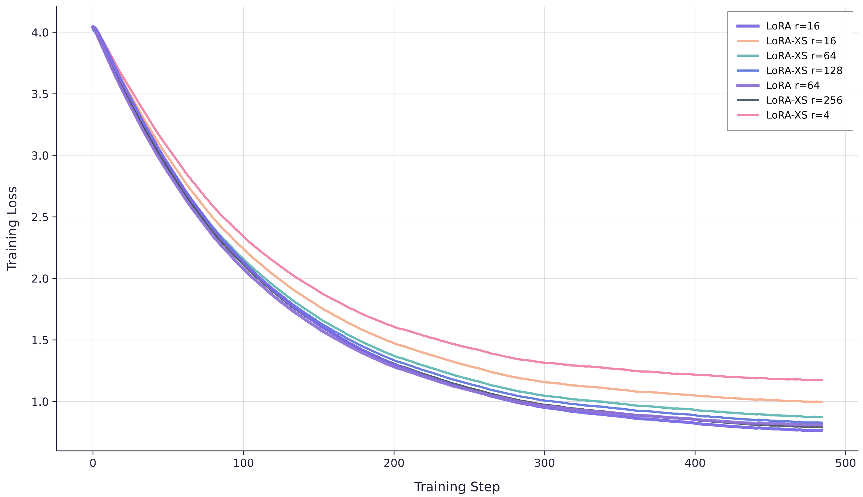
We evaluate LoRA against LoRA-XS on Qwen3-32B, testing four configurations: LoRA rank64 (our baseline, since it performs similarly to ranks 16-256), and LoRA-XS at ranks 64, 128, and 1024. We fix hyperparameters except learning rate, which we tune specifically for LoRA-XS through a sweep from 1e-4 to 7e-3—lower rates caused LoRA-XS to lag significantly behind LoRA, while higher rates introduced instability. We use learning rate 1e-3, $\alpha=32$ for all runs, and batch size 32.

Training curves for LoRA rank64 versus LoRA-XS at ranks 64, 128, and 1024 on Qwen3-32B. LoRA-XS requires rank1024 to match LoRA rank64 performance.
Contrary to the LoRA-XS paper's results, we could not get LoRA-XS to match LoRA performance at ranks 64 or 128. We had to push to rank1024 before matching vanilla LoRA rank64, at which point LoRA-XS has approximately double the trainable parameters. This suggests either a setup mismatch with the original paper (despite careful hyperparameter matching) or that LoRA-XS degrades on larger models, since the paper focused primarily on models up to 8B while we use 32B.
To test whether model size explains the discrepancy, we repeat the experiments on qwen3-4B with the same number of training examples.
Training curves for Qwen3-4B comparing LoRA ranks 16 and 64 against LoRA-XS at ranks 4, 16, 64, 128, and 256. LoRA-XS shows improved but still suboptimal performance.
The 4B results are more encouraging: LoRA-XS rank256 approximates LoRA rank16, though still falls short of the paper's claims. The parameter ratios reveal why smaller models may fare better. For qwen3-32B, LoRA rank16 has 1,986,560 trainable parameters per layer versus LoRA-XS rank256's 458,752 (ratio 4.33:1), while for qwen3-4B the ratio drops to exactly 2:1. This shrinking ratio as models get smaller likely explains why LoRA-XS approaches LoRA performance more closely on 4B than 32B.
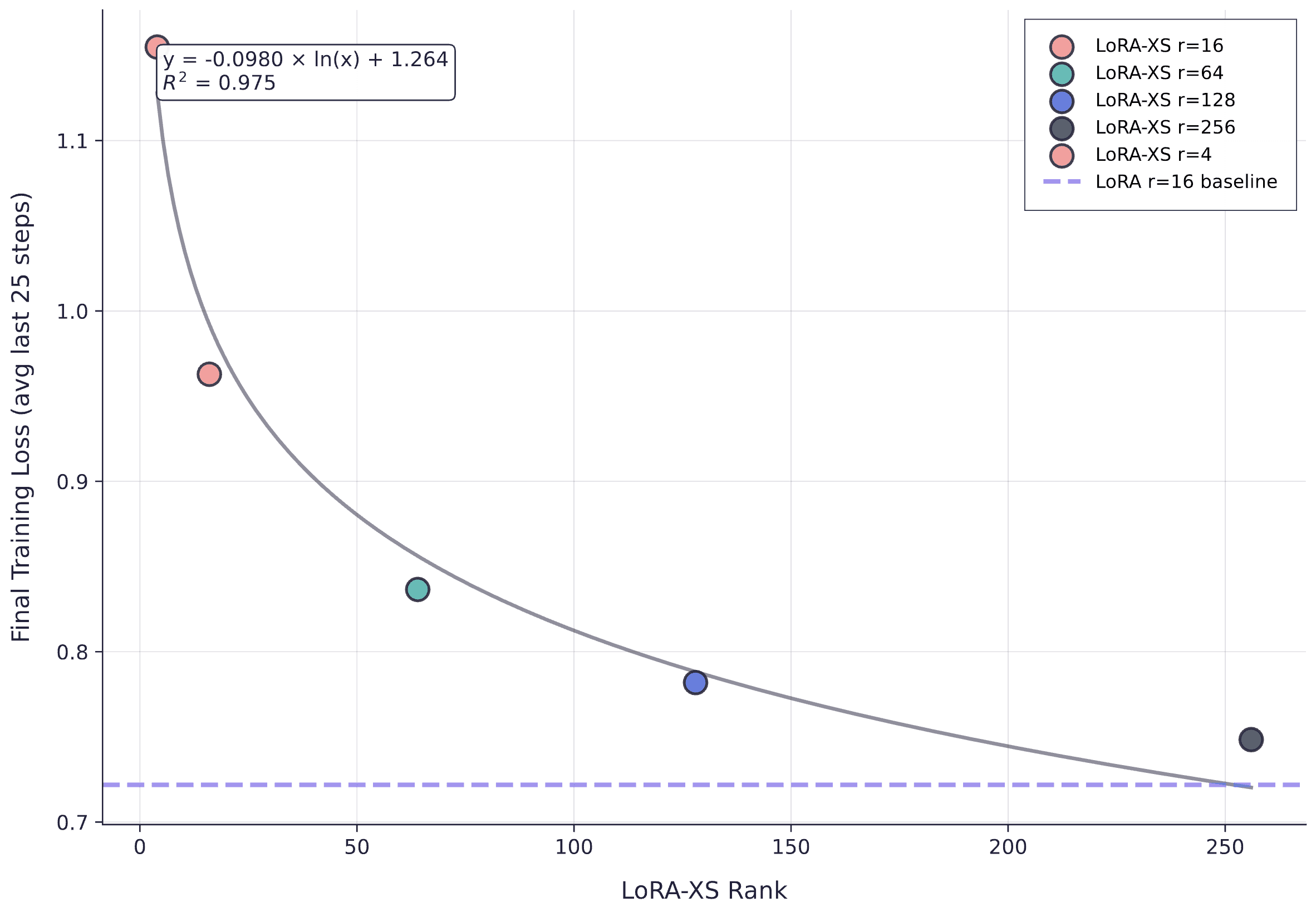
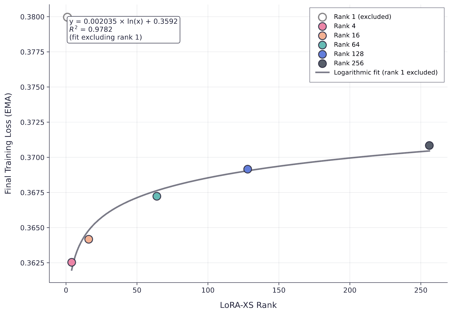
Final training loss versus LoRA-XS rank for Qwen3-4B, with logarithmic fit (R² = 0.975) and LoRA rank16 baseline. LoRA-XS exhibits clear logarithmic scaling but consistently underperforms the LoRA baseline.
The scaling relationship is remarkably clean: final loss decreases logarithmically with LoRA-XS rank, but the entire curve sits above the LoRA baseline, confirming that LoRA-XS requires substantially higher rank than LoRA to achieve equivalent loss.
We also evaluate using our seven LLM-as-judge evaluators (producing scores out of 7) to confirm that loss correlates with downstream performance.
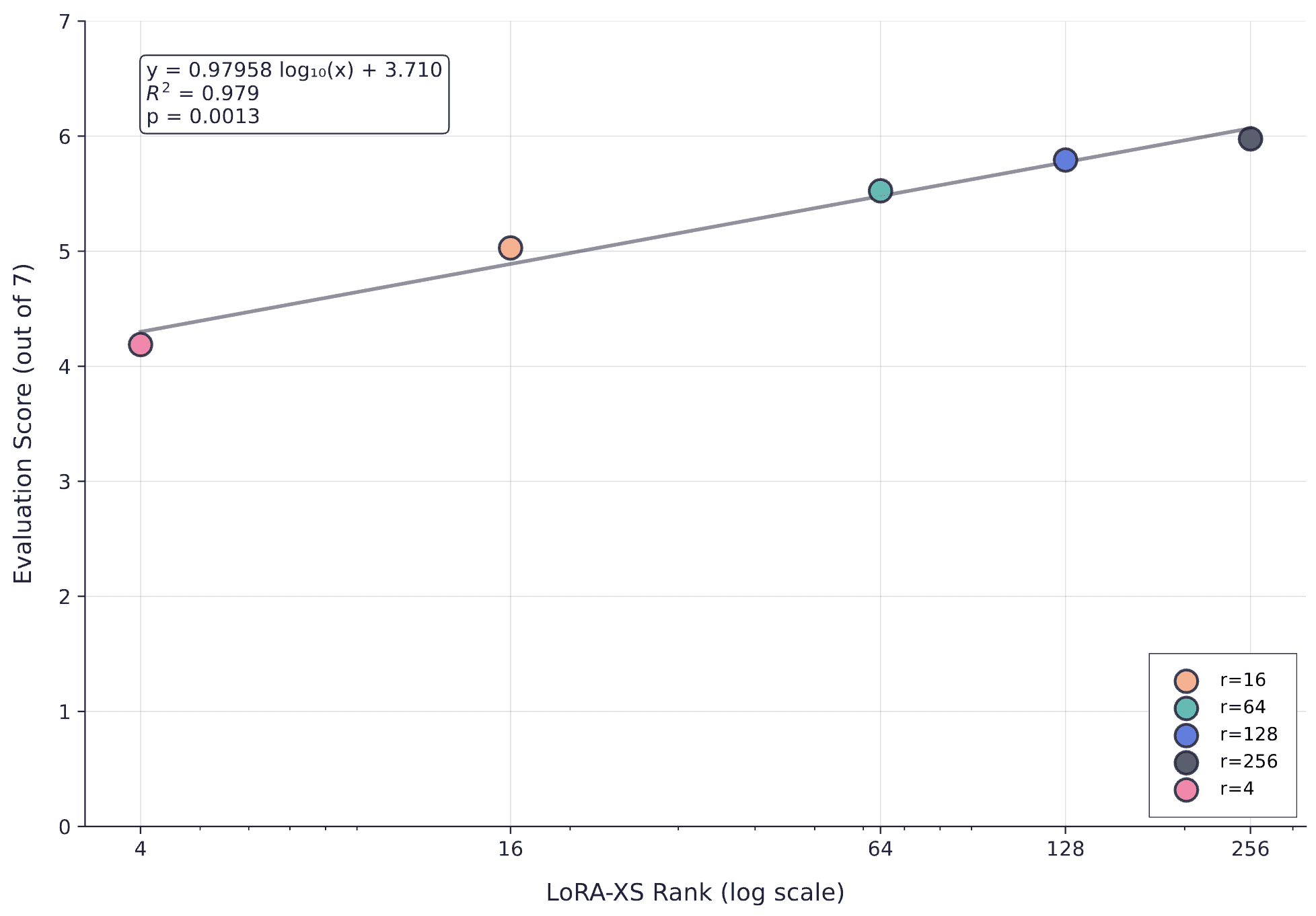
Evaluation score versus LoRA-XS rank (log scale) showing strong logarithmic scaling (R^2 = 0.979, p = 0.0013). The predictable relationship between rank and evaluation score confirms that loss is a reliable proxy for task performance.
Finally, we performed a learning rate sweep for LoRA-XS rank64 on the 4B model to ensure our learning rate choice wasn't the limiting factor.
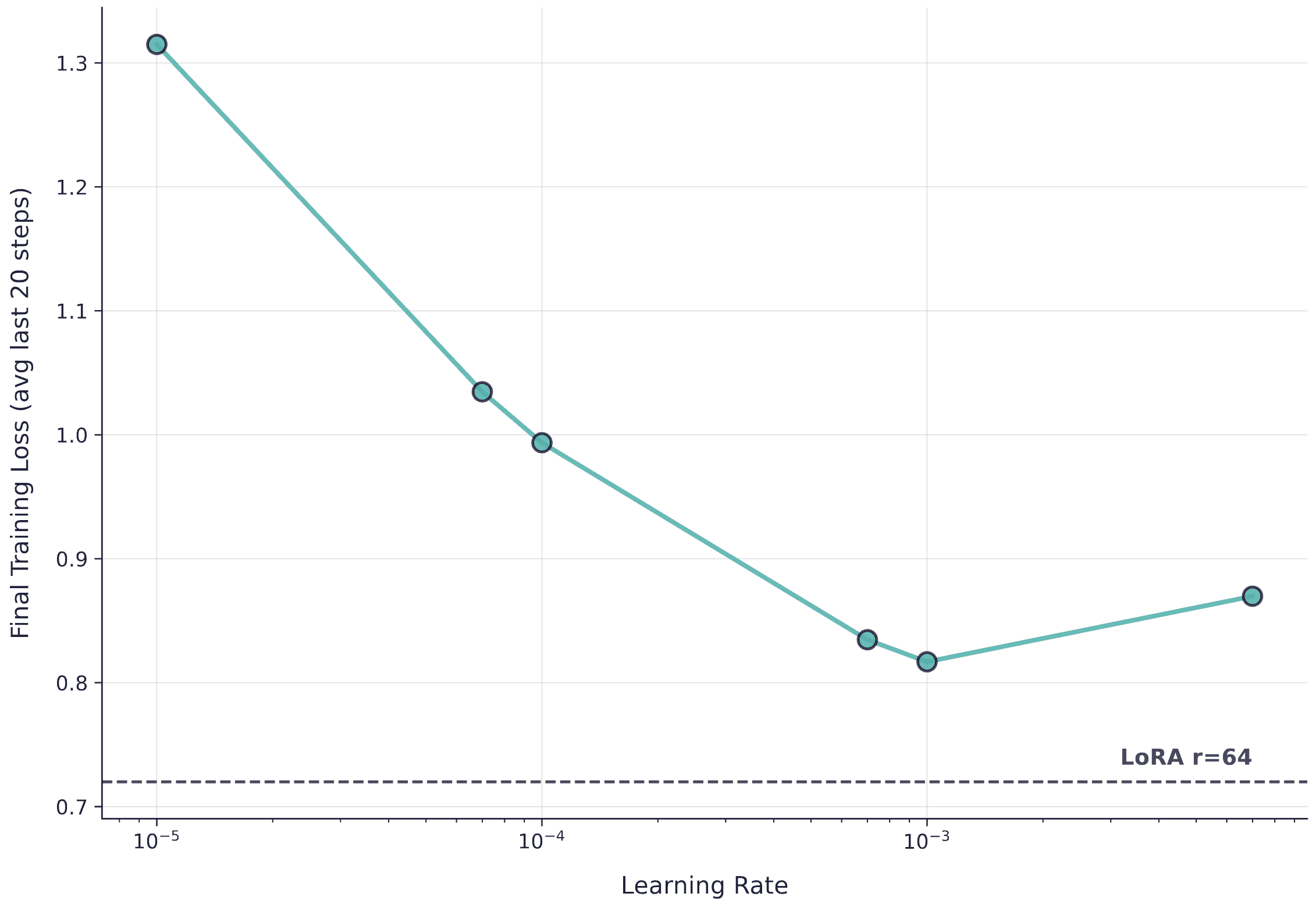
Learning rate sweep for LoRA-XS rank64 on Qwen3-4B, with LoRA rank64 baseline shown as dashed line. No learning rate allows LoRA-XS rank64 to match LoRA rank16 performance.
No learning rate enables LoRA-XS rank64 to surpass even LoRA rank16, let alone rank64. This confirms that the issue isn't learning rate tuning; LoRA-XS genuinely requires much higher rank than the paper suggests to match LoRA on our tasks. For now, we consider LoRA-XS theoretically interesting but practically inferior to standard LoRA for production use.
Initializing LoRA-XS from early updates (and why it didn’t help)
Because LoRA-XS freezes $A$ and $B$ from the truncated SVD of the pre-trained weight $W$ and only learns a tiny square $R$, we asked: what if we first take a few full-FT steps, form $\Delta W=W_{\text{after}}-W_{\text{before}}$, and initialise $A,B$ from the SVD of $\Delta W$ instead? Intuitively, this tries to align LoRA-XS with the actual gradient subspace of the new task rather than with the dominant singular directions of $W$. Concretely: for each adapted matrix we ran a short full-FT “burn-in”, computed
$\Delta W$, set $A=U_r\Sigma_r,\ B=V_r^\top$ from $\Delta W\approx U_r\Sigma_rV_r^\top$,
then froze (A,B) and trained only $R$.
In practice this underperformed our standard LoRA-XS initialization from $W$. The main issue is statistical: a handful of steps gives a noisy, non-stationary estimate of the gradient subspace that is heavily confounded by optimizer state, per-layer scaling, and early-training transients; LoRA-XS’s theory assumes you align with directions that reflect the long-run aggregate of gradients, for which $W$’s top singular vectors are a better proxy than a tiny $\Delta W$ sample. Empirically, the LoRA-XS paper itself recommends (and ablates) SVD-on-$W$ with
$A=U_r\Sigma_r,\ B=V_r^\top$
and finds it generally superior to alternatives, matching our outcome; using $\Delta W$ also produced poorer conditioning of $R$ and occasional instability , while adding burn-in defeats the PEFT objective. We therefore reverted to the paper’s $W$-based initialisation and do not recommend $\Delta W$ initialisation for production.
Discussion
Our results reveal clean scaling laws for LoRA across dataset sizes and ranks, but several subtleties merit deeper examination, particularly around what capacity actually means in practice.
Task structure and intrinsic dimensionality
The saturation analysis above treats “information per token” as roughly uniform, but this obscures a crucial distinction: tasks have wildly different intrinsic dimensionality. A mathematics dataset with varied proof strategies, theorem applications, and reasoning chains occupies a fundamentally higher-rank manifold than most production tasks we encounter. Clinical scribing, for instance, is highly structured: the same template applied to different patient encounters, with bounded variation in medical terminology and note format. Insurance policy recommendations follow similar patterns: repetitive decision trees over a constrained product space.
This means the “bits per token” framing is misleading. What matters isn't raw token count but the entropy of the distribution you're learning. A proof-heavy math task might genuinely require rank 64+ even at modest dataset sizes because the solution space is geometrically complex. Meanwhile, a templated business task might saturate at rank 4-8 even with hundreds of thousands of examples, because the low-rank structure is genuinely capturing most of the variance.
We've observed this empirically but haven't rigorously characterised it. The natural next question is: can we predict required rank from dataset statistics alone? Measuring the effective rank of the input-output joint distribution, or the spectral properties of the empirical gradient covariance, might give us a principled capacity estimator before we even start training. That's an open problem we're actively investigating.
Information flow in fine-tuning
Our capacity calculations assume approximately 1 bit per token, but this is complicated by how we actually compute loss during fine-tuning. We mask user tokens—only assistant tokens contribute to the gradient. Naively, this means user tokens provide zero bits of information, since they don't directly enter the loss.
Obviously this can't be right. User tokens condition the entire assistant response, and the mutual information between (user context, correct assistant response) is substantial. The resolution is that user tokens contribute information through the assistant tokens they condition. In information-theoretic terms: while $I(\text{user tokens}; \text{loss}) = 0$ by construction (they're masked), we have $I(\text{user tokens}; \text{assistant tokens}; \text{model update}) > 0$ through the chain rule of mutual information.
But how much information, precisely? Less than if we'd trained on user tokens directly, certainly. The question is how much less. If you have a dataset of 10M assistant tokens conditioned on 40M user tokens, what's the effective information content? Is it 10M bits (only assistant tokens count)? Or somewhere between 10M and 50M (user tokens contribute but discounted)?
Our working hypothesis is that the effective information scales with the entropy of the conditional distribution $p(\text{assistant} | \text{user})$, not the raw token counts. For highly deterministic tasks (scribing a medical note has low entropy given the transcript), this could be substantially less than 1 bit per assistant token. For creative or reasoning tasks, it might approach the full token count.
This also explains why pretraining is so different. During pretraining, every token contributes to loss, and the prediction task is genuinely high-entropy (next token is highly uncertain given current context). Fine-tuning on narrow distributions should saturate adapters much faster than pretraining would, which is exactly what we and Thinking Machines observe.
What we've learned at scale
The experiments above use datasets up to 30K examples, which is instructive but small by production standards. We've run extensive tests on customer datasets with 100K-1M+ examples of ~15K tokens each (hundreds of millions of tokens total), but cannot share these results due to privacy commitments.
We can say that the fundamental patterns hold. The logarithmic rank-loss relationship persists. Capacity saturation follows similar dynamics, just shifted to higher token counts and sometimes requiring higher ranks. For our most data-rich customers, we routinely use rank 16-64 and still see clean convergence without saturation effects, suggesting the real capacity limits for these tasks are comfortably above what we've hit.
Future work: rigorous characterisation at scale
The loss-evaluation correlation we showed is suggestive but not definitive. We need more statistical power to confidently use loss as a checkpointing proxy, which requires systematic experiments across multiple tasks, dataset sizes, and evaluation metrics. We're currently running these studies on tasks where we can roughly understand entropy (by looking at the final loss of a really big, full fine-tuned model) then validating on production data. The goal is a quantitative model that predicts: given task X with measured properties Y, rank r will saturate at Z tokens with confidence intervals.
We're also investigating whether low-rank training exhibits different generalisation properties than full fine-tuning, even when loss matches. LoRA constrains the update to a low-dimensional subspace: does this act as implicit regularisation? (Recently, a paper showed that fine-tuning methods which minimised KL divergence to the base model mitigated catastrophic forgetting - does LoRA help with this?) Do we get better out-of-distribution performance, or worse? Initial signals are mixed and likely task-dependent, but it's worth systematic study (to us anyway).
Multi-tenancy and production inference
One compelling reason for using LoRA is multi-tenant serving: storing a single base model and swapping adapters per request, letting us serve multiple distinct customer models on one node instead of replicating the base model for each. The key insight is that you don't actually "swap" adapters in the sense of loading/unloading them—instead, you compute the base model output once for the entire batch, then group requests by adapter and compute each adapter's contribution separately, adding the results back to the base output at the appropriate indices.
This works because LoRA’s forward pass can be computed as $Wx + B(Ax)$ rather than materialising the full update $\Delta W = BA$ first. For a weight matrix $W \in \mathbb{R}^{d \times k}$ with LoRA matrices $A \in \mathbb{R}^{r \times k}$ and $B \in \mathbb{R}^{d \times r}$, applying the factored form costs $O(rk + dr)$ operations per token, whereas applying a pre-materialised $BA$ would cost $O(dk)$ per token (and forming $BA$ would be a one-off $O(drk)$ cost we avoid). When $r \ll \min(d,k)$ this is much cheaper: with $d = k = 4096$ and $r = 16$, the factored form is $\sim 131K$ MACs vs $\sim 16.8M$ MACs for $(BA)x$, a $\sim 128\times$ improvement. The batched computation amortises the base path across all requests while keeping adapter-specific work small and grouped.
vLLM already supports this pattern through segmented batched GEMMs and unified paging for adapter weights, and we're currently integrating similar optimizations into our forked inference engine. The memory hierarchy is straightforward: base model weights stay resident, adapter weights (A and B matrices, typically ~200MB per adapter for rank-16 on a 7B model) are paged in/out of GPU memory as needed, and a request scheduler groups incoming requests by adapter ID to maximise batching efficiency. The challenge isn't latency from memory movement—it's building the batching logic and memory management to handle dynamic adapter access patterns without fragmenting GPU memory or breaking batch cohesion.
Closing thoughts
LoRA works remarkably well when you get the details right, and the scaling laws are clean enough to be predictive. LoRA-XS remains an interesting idea that doesn't (yet) deliver in practice, at least not for our workloads at our scales. The theoretical foundations are sound, but somewhere between theory and practice, the gains evaporate.
For practitioners: use rank 8-16 as default, scale up to rank 32 if you have evidence of saturation, and don't bother with rank 4 unless you're severely memory-constrained. Measure loss carefully, trust it as a leading indicator of eval performance, and checkpoint aggressively. The parameter savings (ie memory, particularly from the optimiser states) are real and the quality is equivalent to full fine-tuning (in the regimes we care about).
We're continuing to push on the fundamentals. Understanding when and why low-rank methods work is directly actionable for building better production systems.