Attention-based attribution: what your model is actually looking at

Auditability, explainability and interpretability are often thrown around as buzzwords in the generative AI space. For instance, some clinical scribes claim to offer something called attribution: for any given chunk of text in the model’s output, what were the chunks of text in the input that most “influenced” this part of the generation?

However, the definition of influence in this context can be very nebulous. For instance, if a company (such as the above scribe) are using closed-source models, and all you get back from the API is text, then how do you compute influence? Well, really your only option is to chunk up the text, and then look at the similarity of a chunk in the output to the chunks in the input. Typically, this is done by embedding the chunks (with an encoder transformer, such as OpenAI’s text-embedding-3-small) and calculating the cosine similarity between chunks.

This, we stress, is not influence. It’s a useful similarity measure, but it’s not telling you at all what the model was actually doing when it generated that chunk. Worse than that, it’s not very good. Specifically, when you’re creating some quantitative representation of a chunk of text (like an embedding) you only represent information present in that actual chunk, devoid of the context of the information preceding and after it. We’ll look at a specific example of where this fails for cosine similarity below, but the overall message is: don’t trust a company at all when they tell you they’re giving you attribution and auditability. What they’re giving you is a hacked-together arbitrary similarity measure that is not derived from the actual model doing the generation. To do true explainability, you need access to the model internals. Fortunately, since we fine-tune open-source models at Parsed, this is exactly something that we can do.

Where cosine similarity fails

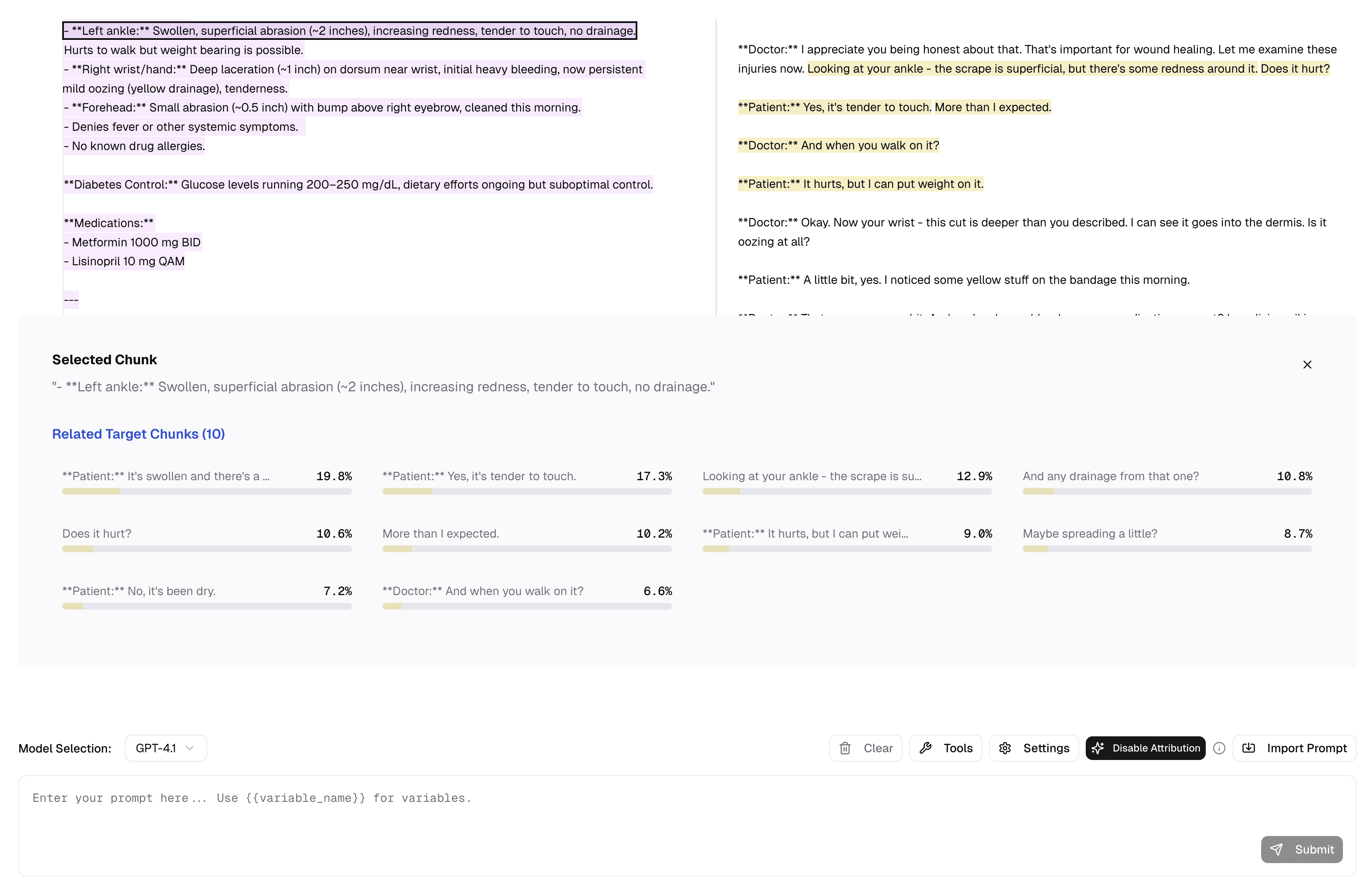
Let’s look at a simple task: a model is given a transcript, and instructed to generate a clinical note, much like a doctor would write. We note that the model has written a list of three injuries: an ankle abrasion, a wrist laceration, and a forehead contusion. One thing attribution is really useful for is visualising where a model might have taken the information from in the input in order to generate a particular part of an output. We might do this, for instance, to check if a model hallucinated some part of its generation, or if it did indeed generate it based on information in the input.

Let’s start by looking at cosine similarity on this synthetic example. Where does it think the information came from? Again, recall that to get the attribution score for this particular “chunk” of the output, we simply embed the output chunk, and embed all the input chunks, and calculate the cosine similarity between the input-output chunk pairs. (For the sake of this example, we chunk just on new lines and full stops.) Here’s what cosine similarity looks like (ie the top three chunks attributable to the output chunk we’ve selected):

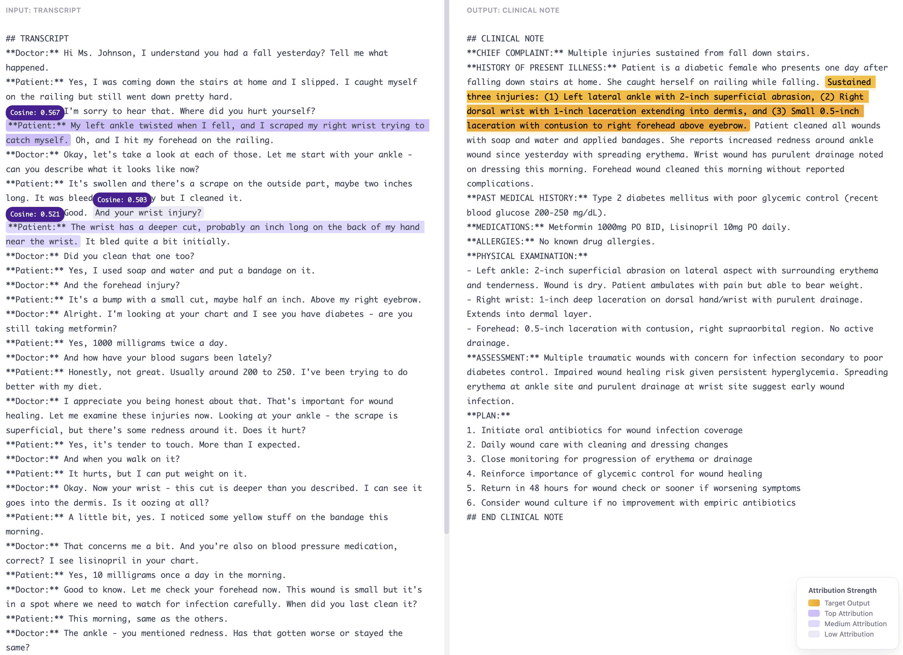
Cosine similarity completely misses the third wound (the forehead wound)! It’s clear why cosine similarity misses this information. Because the embedding for a particular chunk can only contain information localised to that chunk, it doesn’t have the versatility to understand that this third injury is referring to the forehead, which comes earlier in the transcript (”And the forehead injury?”)

Now, let’s see if attention does any better. He, we pick a single layer of the pre-trained transformer qwen3-32b (layer 40) and calculate the attention heatmap by averaging the attention over the heads in the layer, and aggregating attention across chunks.

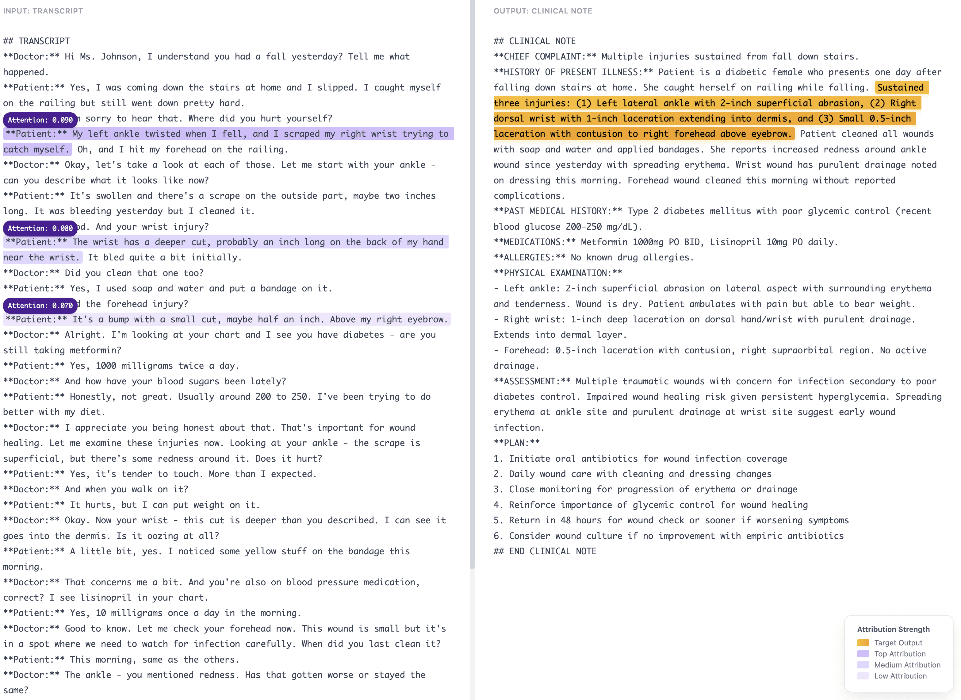
Attention gets it! It understands that “It’s a bump with a small cut” refers to the forehead injury, because the attention information is not just localised to that particular chunk - by definition, attention uses the context of everything that has come before it to figure out where to look. This is a very simple and contrived example, but hopefully it gives some intuition of why cosine similarity often breaks down, and where attention can improve on it.

Developing attention attribution into a useful tool

Of course, once you understand how attention works, it’s the most obvious thing in the world that we’d want to use this to do attribution. However, there are still a lot of choices we need to make. First, we must decide whether to extract attention from the actual generating model (providing ground-truth attribution but requiring significant computational overhead) or from a smaller proxy model (trading some accuracy for efficiency). If using a proxy model, we need to determine: Which model size provides sufficient attention fidelity? Which specific layers capture the most relevant attention patterns? And crucially, what's the minimal subset of layers that maintains high correlation with full-model attention while remaining computationally feasible?

We also have some real-world engineering constraints. In a live inference setting, attribution must add negligible latency (< 100ms) to maintain responsive user experience—ruling out complex post-processing like iterative attention sink normalisation that can take seconds on long contexts (although we still do some form of attention sink normalisation). More critically, during generation, our GPUs operate at near-maximum memory utilisation to maximise throughput; storing full attention tensors for a 70B parameter model with 80 layers would require ~10-50GB of additional memory per request (depending on sequence length), which would force us to reduce batch sizes and directly impact serving capacity. These constraints drove our architectural decision: we decouple attribution from generation entirely, running a dedicated attribution model on separate, smaller GPUs. This separation allows us to optimise each system independently: the generation cluster for maximum throughput, and the attribution system for memory-efficient attention extraction using only the most informative layers (typically 10-15 layers rather than all 80), reducing memory requirements by 5-8x while maintaining >0.9 correlation with full-model attention patterns.

Establishing a ground-truth

We began by approaching the problem practically. Unfortunately, you can’t just use all the attention layers from a model to get something meaningful, because different layers focus on different things. Much like the layers in CNNs focus on increasingly abstract concepts (looking at things like colours and lines in early layers, onto more complex patterns in the middle layers through to abstract concepts like “dog ear” in the later layers), transformer attention patterns follow a similar ascending complexity. Earlier layers tend to focus on grammatical structures, whereas later layers start to look at semantically related information relevant to the current token its attending to. Simply averaging across all layers would conflate these distinct attention types, obscuring the semantic attribution signal with syntactic noise from early layers and over-specialised task features from final layers.

We did this in a pretty practical way. We got a team of doctors (led by our CEO and ex-doctor, Mudith) to do blind A/B tests with different model layers and subsets of layers, to see which points maximised the “intuitive agreement” with the model attention. We found that layers from about halfway through the model up until a couple of layers before the final layer worked best and provided what seemed to be the most understandable view of where the model was looking. These experiments were done on both gemma-3-27b and qwen3-32b models. Although not entirely principled, we choose layers 40-60 in the qwen3-32b model as the ground-truth attention source (averaging over both layers and attention heads in each of those layers). All correlations and comparisons are based on this. We discuss more wholistic derivations of how to get out the full attention information in the appendix, and the drawbacks of doing so.

Measuring Chunk-Level Attention Similarity

We employ three complementary metrics to quantify how well a smaller model's chunk-to-chunk attention patterns match the 32B reference model. RMSE provides an overall element-wise distance measure, treating the attention matrix as a whole and computing the L2 norm of differences. Maximum Jensen-Shannon Divergence (Max JSD) evaluates the worst-case distributional difference across rows, treating each target chunk's attention distribution over source chunks as a probability distribution and computing the symmetric KL divergence, then taking the maximum across all rows to identify the most problematic target chunk. Minimum Spearman ρ (Min Spearman ρ) captures rank-order correlation by computing the Spearman correlation coefficient for each row independently (testing whether chunks attend to sources in the same relative order) and reporting the minimum to identify where ranking breaks down most severely.

Correlation across model sizes

The first thing we want to look at is whether smaller models can approximate the attention of the larger, ground-truth model (say, the model doing the generating). To do this, we take the same relative slice of layers (ie layers 0.6-0.9 through the model) and average the attention across heads and layers. Interestingly, we can get quite close to qwen3-32b with the 14B and even 7B model.

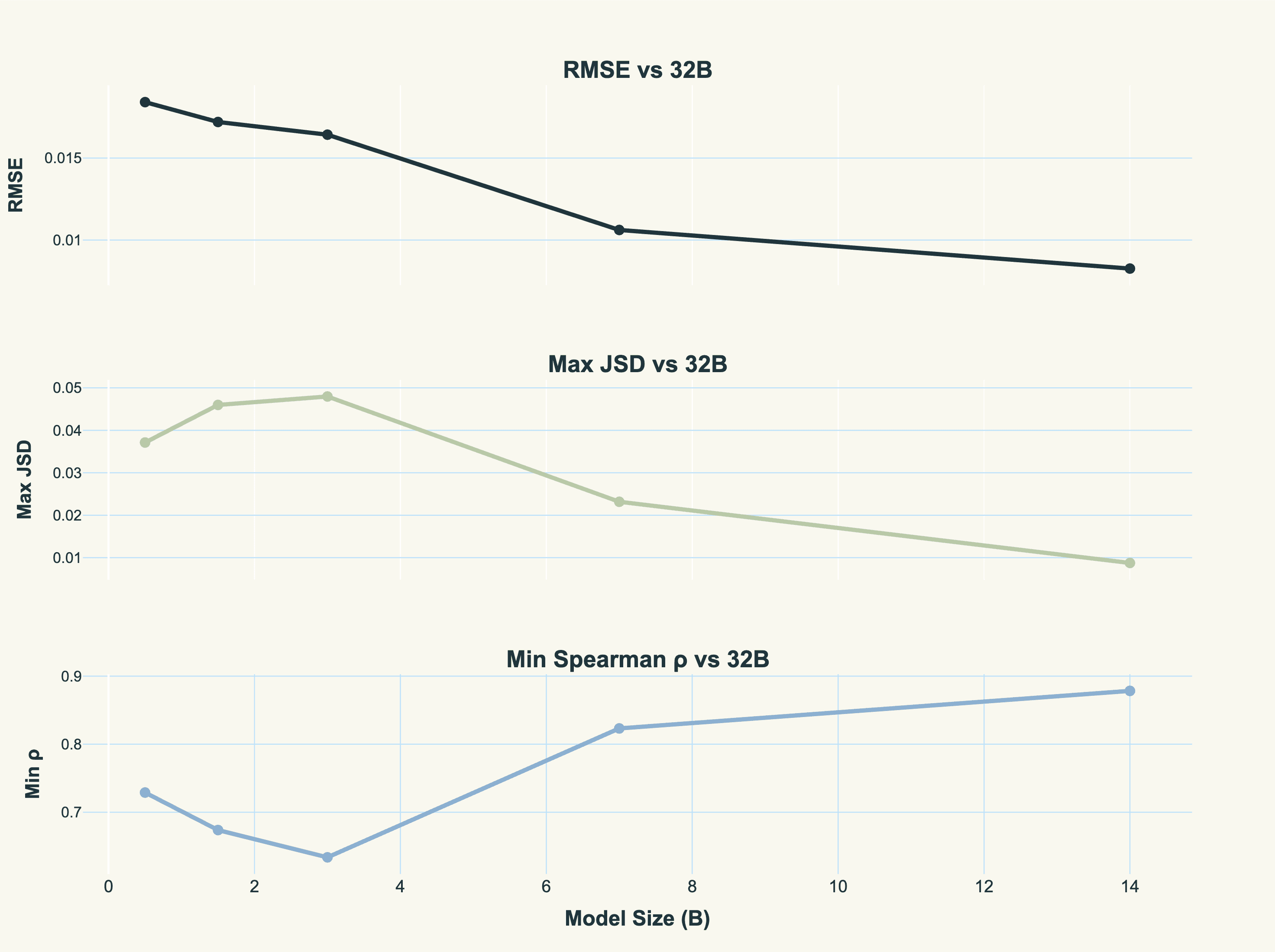
It’s also interesting that there is a drop off in similarity from 0.5B to 1.5B to 3B. This is possibly because the fractional relative slice of layers is not well calibrated for these models, but also because the qwen models are weird in that they don’t monotonically increase in depth as you go up the model family.

Regardless, most of the middle to later layers in the semi-large models have good correlation with the ground-truth from the 32B model.

Correlation across subsets of model layers

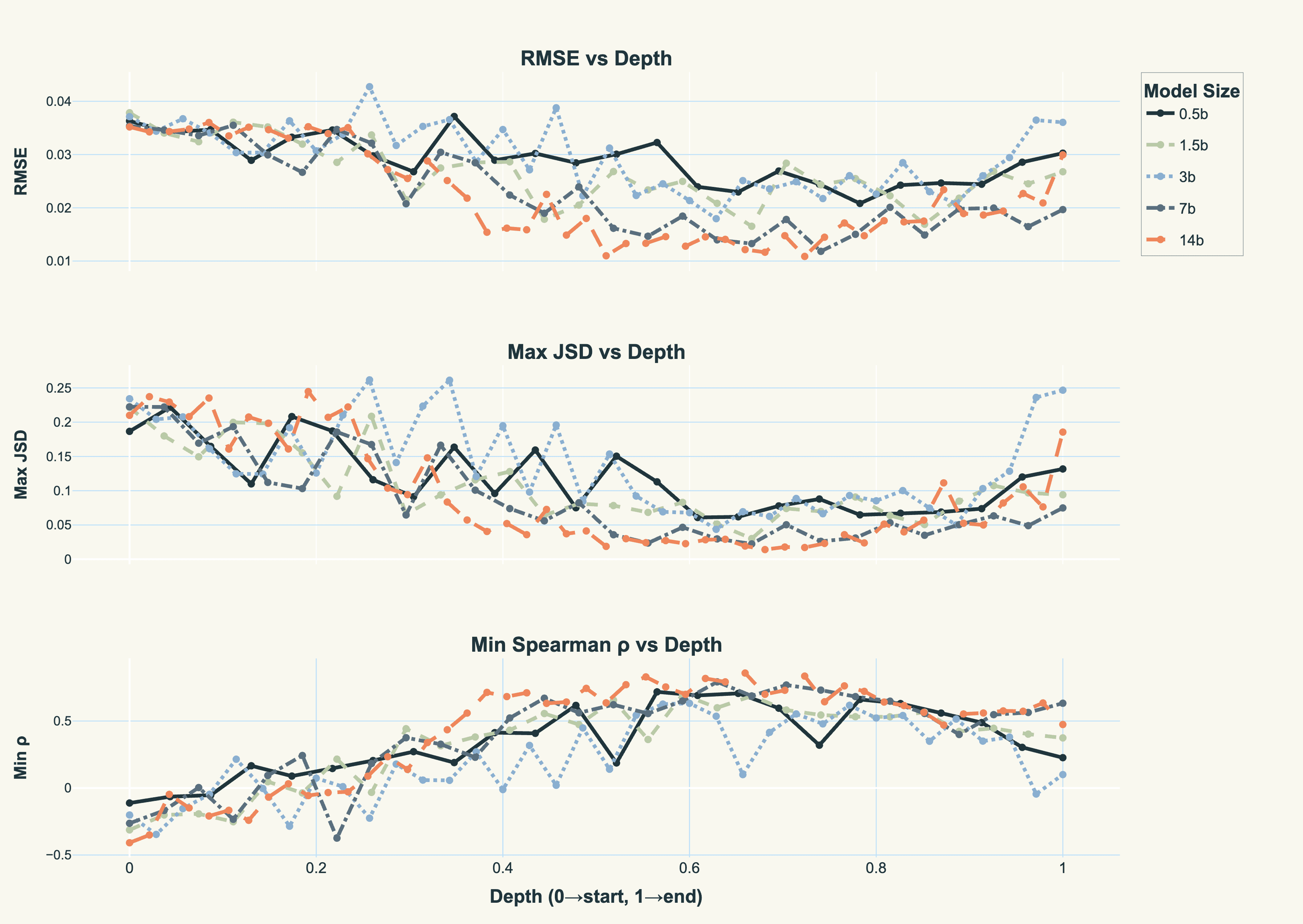
Of course, another way to trade off memory and compute is by only using a subset of layers from the same model (ie from qwen3-32b). To look at which are the best layers to pick, we can calculate the same statistics by comparing the attention patterns of an individual layer to the “ground-truth” aggregated attention patterns.

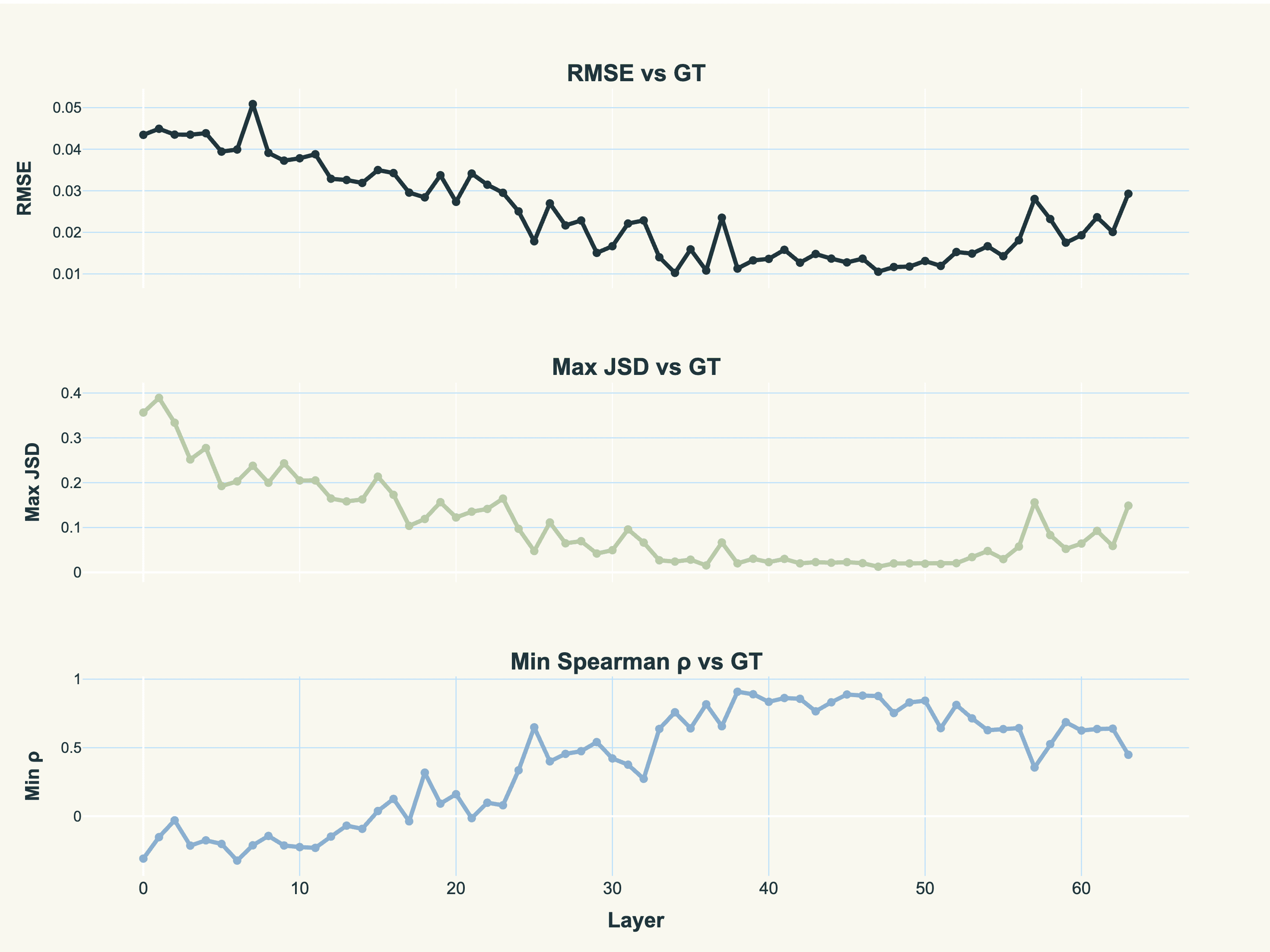
Clearly, most layers in the range we actually picked (39-58) correlate quite well with the averaged attention, suggesting it doesn’t vary that much. This is great! It means we can get away with a subset of layers, possibly even as few as 1-3.

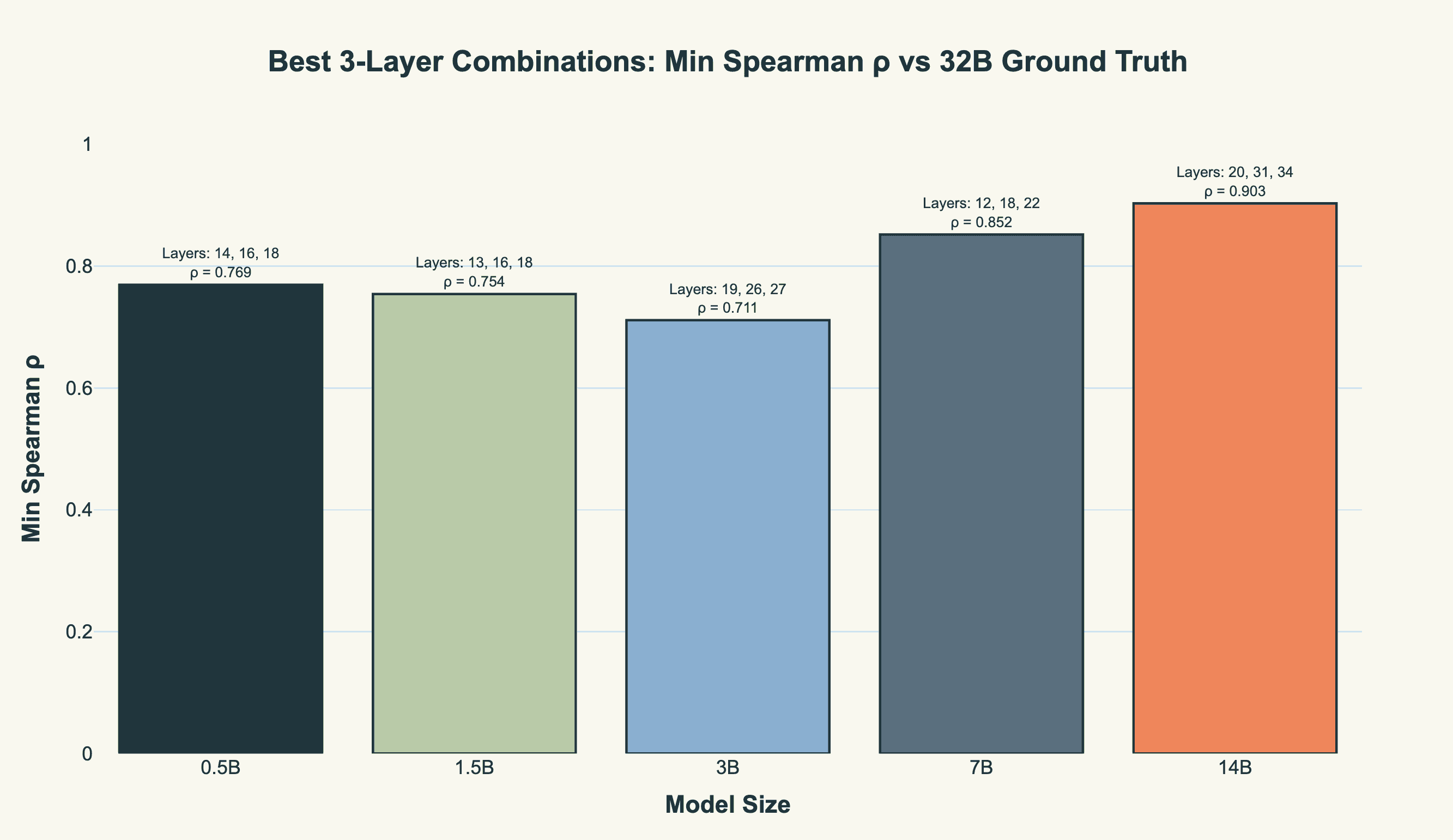
Let’s say we have enough compute on the instance to be able to do 3 layers comfortably. We can also do a search over all the permutations of layers that lead to the highest correlation, across models.

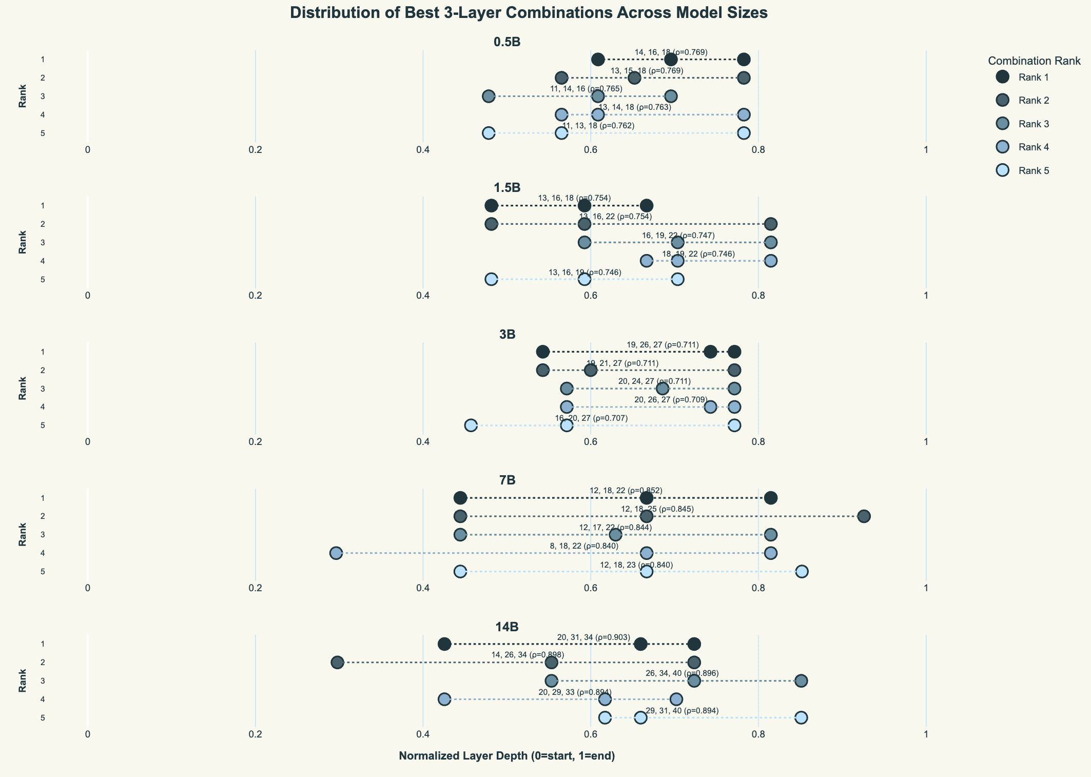
A better way to visualise this is to show the distribution of the top 5 layer choices, across the models. We again normalise the layer depth. The spread is roughly the same - about halfway through the model, roughly evenly spaced, ending about four-fifths through the layers.

In practice, we use a collection of these automated analyses and heuristics when we are attributing with a new model to choose the best subset of layers and best model to approximate the “ground-truth” attention. However, important to note is that some customers need the ground-truth for regulation or compliance purposes, in which case we use the actual model that does the generation and essentially the full layers end-to-end (see Appendix for a discussion of this).

Attention attribution in the Parsed platform

The best part of all this is that it’s live in the Parsed platform! Our customers not only get access to fine-tuned models optimised for their task, but they can also get attribution information. We usually send this back via our API, but here we show visually what attribution looks like in the Playground. Importantly, we can also use any closed-source model and use attention to generate attributions for it (which is useful here where we can’t publicly display an individual customer’s model, but in general allows us to attribution on arbitrary pieces of text):

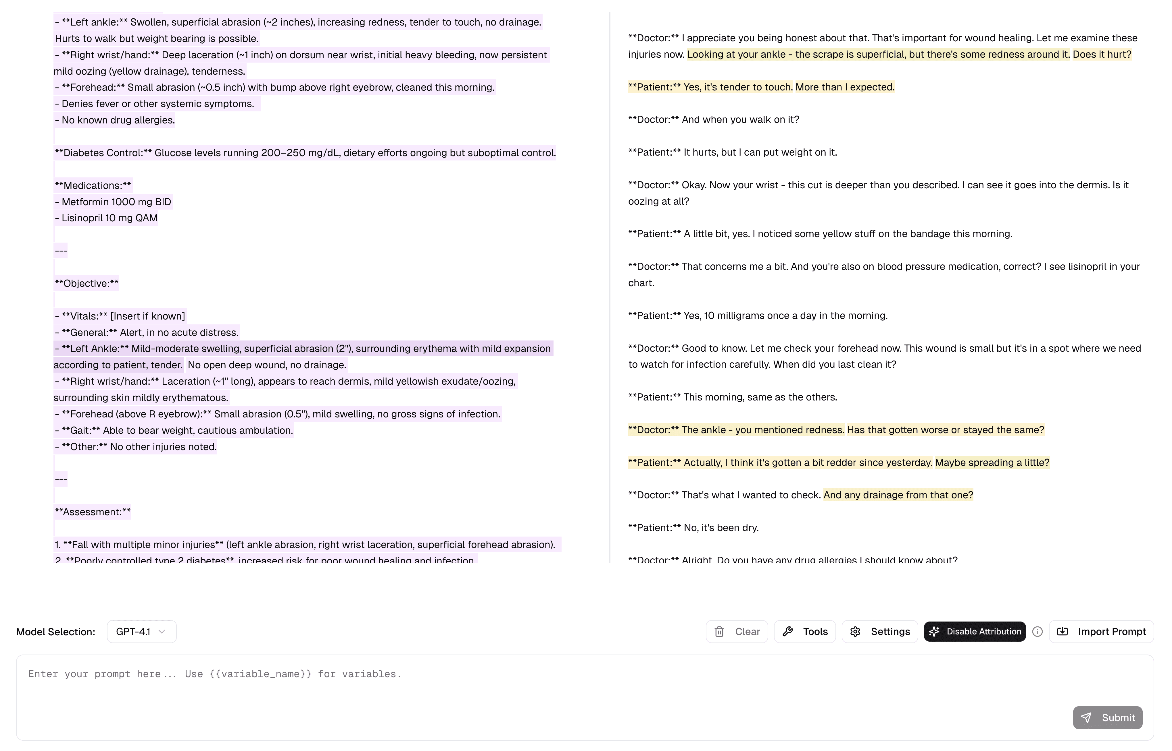
We can also click on any particular output chunk, and see the related target chunks in the input in a popup. Clicking on any of these related chunks will take you to the point in the input where that target chunk is located.

Our customers use this in a variety of circumstances:

• Internal engineering teams use it to quickly sanity-check the outputs of models

• Quality-assurance/internal annotation and labelling teams (such as the medical knowledge teams in our scribe customers) use it as a very efficient way of seeing if the model has used the information in the input correctly, and whether there are parts of the output that are hallucinated (ie not derived from) the input

• Passing through the attribution information returned in our API to end-users and building their own frontends around it. For instance, some of our scribe customers have built the attribution hover-and-click mechanisms into their platforms so that doctors themselves can quickly scan and see where the model was looking for particular parts of the notes.

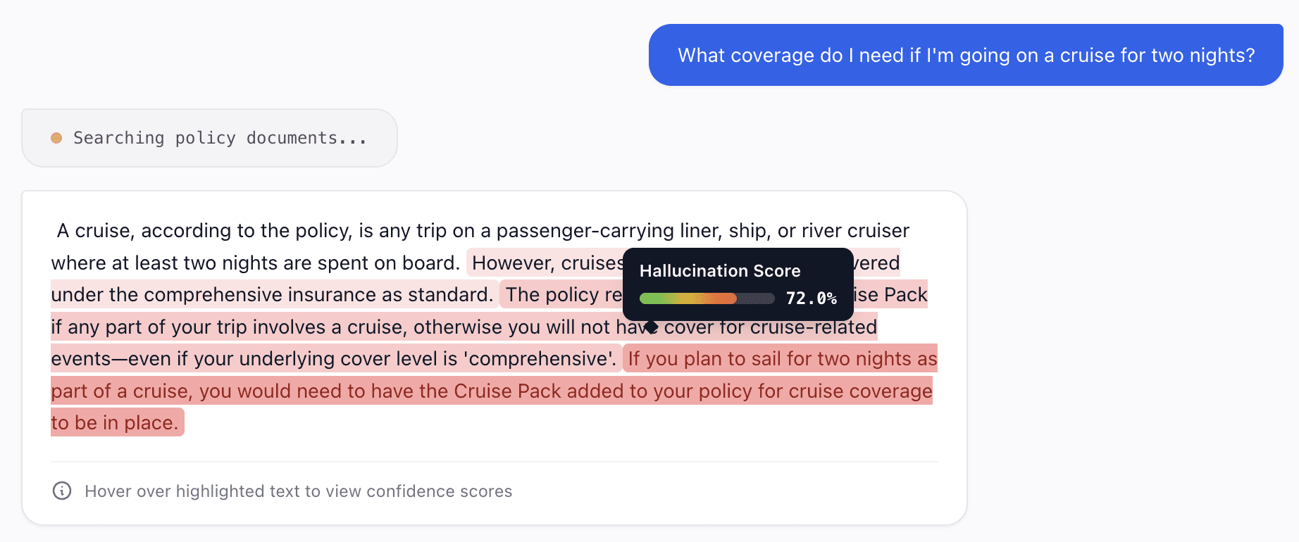
Of course, such ground-truth auditability is useful in a large number of domains. Healthcare (particularly scribes) are obviously useful places to apply this, but in addition another place where interpretability has found a home is insurance. Here, it’s so important that the model only use information from provided policy documents, for instance, and not its own knowledge. Attention attribution is a much more fail-safe way to check for this, as opposed to LLM-as-judge or cosine-similarity-based attribution.

Future work

One might imagine the garden of useful mechanistic interpretability techniques to be a ladder of increasing complexity. Attention attribution is quite simple and is thus quite a low rung on this ladder. Motivated by using attention (or any model internals) to diagnose hallucinations at a chunk-level in model outputs, we asked ourselves: what if we used model internals to try and predict if a particular chunk is hallucinated (ie not supported by the input context) or not?

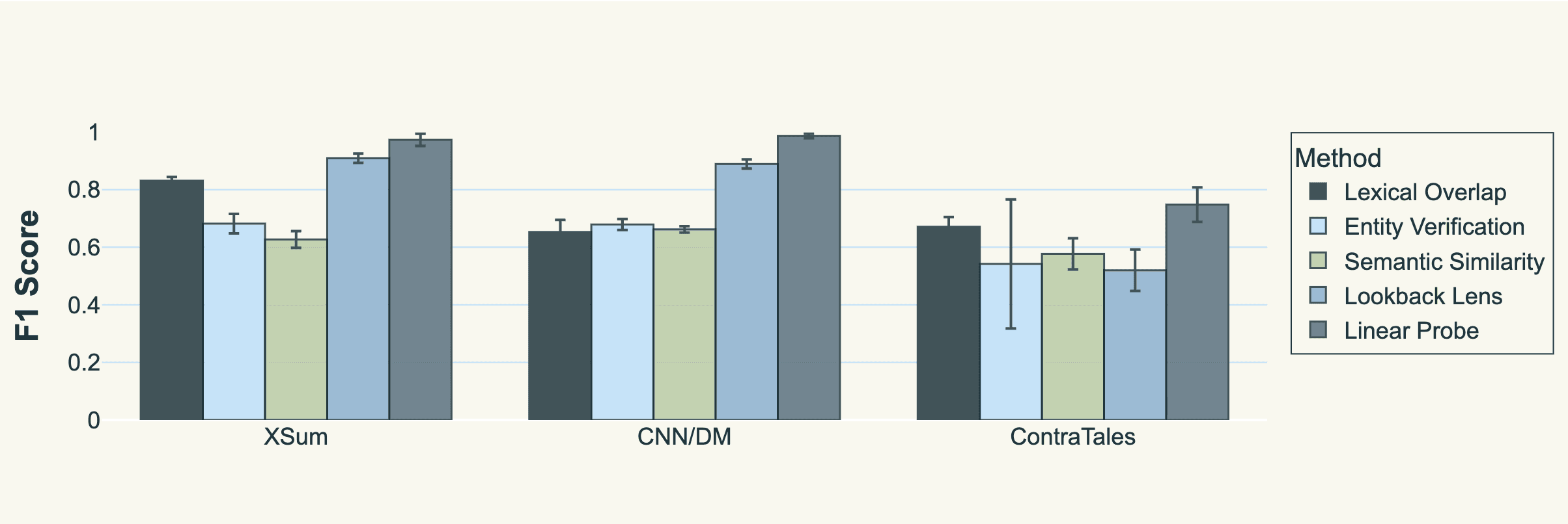
We initially thought we might be able to do this by training lightweight classifiers over the attention matrices themselves (an extension of ideas such as Lookback Lens) but found that training these same linear probes on the residual stream of the transformer (where the model “stores” all its intermediate computations) worked best. We published a paper on this at ICML, where we showed that not only can we, with high accuracy, predict whether a particular generated chunk was hallucinated by using the same model that generated it, but that we could actually take any model’s generation and use a fixed “judge” model’s internal activations to predict whether a particular chunk was hallucinated (ie whether it was supported by preceding input or not). This simple method outperformed all other approaches we tried, including semantic similarity (cosine-similarity), lexical overlap, entity verification and lookback lens.

This allows us to do cool stuff like flagging hallucinations live as we send back responses to customers. Whilst this is only available in the API currently, one might imagine being able to display this information in a similar manner to how we display attribution scores.

Another useful direction we’ve been looking into is trying to answer the following question. Suppose we have a fine-tuned model which is really good at doing a particular task (say generating clinical notes). What is the difference between the attention this model pays to parts of the input, and the attention of the base (not fine-tuned) version of the model? If the attention is exactly the same, then we can serve our attention attribution more efficiently by using one base model deployment for all customers using attention attribution. Our initial hypothesis is that they’re quite similar, supported by evidence such as the fact that fine-tuning LoRA adapters on attention components only does not really increase performance, so a lot of the updates are probably confined to the MLPs. This is something we’re actively investigating.

Finally, we are also looking at methods which better approximate the full model attention across layers, taking into account the mixing of information from different tokens. We discuss this in the Appendix.

Appendix

A more principled derivation

While individual attention matrices show local token-to-token relationships at each layer, they don't capture the full picture of how information propagates through the network's depth. This appendix derives a principled method for computing the total effective attention from input to output, accounting for both attention mechanisms and residual connections.

The model

At each layer l, the transformer computes:

For attention-only analysis (ignoring MLPs), we can linearise this as:

where

is the attention weight from token i to token j at layer l, and I is the identity matrix representing the residual connection.

To understand how information flows from input (h^0) to layer L, we compose these transformations:

Expanding this product reveals how information propagates through multiple paths:

• Direct paths: Information flowing straight through residual connections

  

• Single-hop paths: Information modified by attention at exactly one layer

• Multi-hop paths: Information transformed by attention at multiple layers

The effective attention matrix that captures all information from input to output is:

Subtracting I removes the direct residual path, leaving only the attention-mediated influence.

However, we find that this doesn’t necessarily provide the most useful attention patterns. What ends up happening is that everything converges to a small set of input chunks, and there is not a huge amount of variance in these input chunks. This is probably because earlier layers again have high attention on grammatical tokens (”the”, “.”, etc) and this converges to a pretty sparse attention pattern. We can run this process in theory on just the layers we care about (ie the layers we chose above to average for qwen3-32b) and this is something we’re looking into as to whether this ends up better.

(Upon deriving the above, we realised this had been done before in this paper.)

What exactly should A^l be?

Here, we set A^l to raw attention probabilities (averaged over heads), and the product is thus the classic attention rollout heuristic. It captures routing structure, but not the magnitude effects of value and output projections, layer norms, etc.

If we wanted a more quantitatively faithful “influence”, the principled object is the token-to-token Jacobian of the attention block at the input we care about:

and then

Attention sink normalisation

To address the phenomenon of attention sinks (tokens that accumulate disproportionately high attention weights regardless of semantic relevance) we implement a statistical outlier detection approach. For each output token position, we extract its attention distribution over all preceding input tokens and compute the median attention value across the output sequence. We then apply a log transformation (with a small constant added to prevent numerical instability: log(attention + min/2)) to better capture the heavy-tailed distribution of attention weights. Tokens are identified as attention sinks when their log-transformed attention exceeds μ + 3σ, where μ and σ are the mean and standard deviation of the log-attention distribution. These identified sink tokens can then be masked or down-weighted during attribution analysis. This approach effectively identifies grammatical tokens and separators that accumulate excessive attention (typically punctuation, articles, and structural tokens).